The Retrieval Stage: Finding and Filtering Candidates

The goal of this stage is simple in theory but complex in practice: from a corpus of millions or even billions of items, produce a slate of around 500-1000 candidates that is highly likely to contain the "perfect" items for a given user. This has to happen in tens of milliseconds. Precision isn't the primary goal here; recall is. We want to cast a wide but intelligent net, ensuring we don't prematurely discard the items that would have scored highest in our perfect, impossible oracle function.

Offline Preparation: The Foundation of Speed

The speed of the online retrieval stage is bought with offline compute. This is a fundamental trade-off in large-scale systems. The heavy, time-consuming work is done beforehand, producing artifacts that can be served quickly at request time.

Before a single user request is handled, the retrieval stage relies on several key offline processes:

1. Model Training: If we're using model-based retrieval (like a Two-Tower network), the models are trained offline on historical interaction data.
2. Embedding Generation: The trained models are then used to compute a d-dimensional embedding vector for every single item in the corpus. This can be a massive batch computation that runs daily or weekly.
3. Indexing: These generated artifacts are then indexed for fast lookup. This is the most critical step for online performance.
   
   • ANN Indexes: Item embeddings are loaded into an Approximate Nearest Neighbor (ANN) index using libraries like FAISS or ScaNN. This allows us to find the "closest" item vectors to a given query vector in sub-linear time, trading a small amount of accuracy for a massive gain in speed.
   • Inverted Indexes: Item metadata is loaded into an inverted index (like those used by Elasticsearch or Lucene) to enable fast attribute-based filtering.
4. Preparing Heuristic Data: Simple lists, like the "top 100 most popular items of the week," are pre-calculated and stored in a key-value store (like Redis) for fast access.

The Online Request Flow: A Three-Step Process

When a user request comes in, the retrieval stage executes a fast, sequential process.

Step 1: Pre-Filtering: The Cheapest Win

The most effective way to reduce latency and cost is to reduce the search space before running any expensive candidate generation logic. Pre-filtering applies hard, binary constraints based on the request context.

A classic example is a food delivery app. If a user is searching for a restaurant, the system can apply several pre-filters:

• is_open = true
• delivers_to = user_zip_code
• max_delivery_time < 45_minutes

These filters are typically executed against a metadata store or an inverted index, reducing a potential pool of tens of thousands of restaurants to just a few hundred. Only this much smaller set is then passed to the candidate generation models.

Step 2: Candidate Generation: The Ensemble

No single retriever is perfect. Production systems almost always use an ensemble of retrievers, running multiple candidate generation strategies in parallel and blending their results. Each retriever has different strengths, and together they create a more robust and comprehensive candidate set.

Here are the most common types:

1. Heuristic Retrievers These are simple, rule-based sources that are cheap to implement and serve. They are surprisingly effective, especially for solving the cold-start problem and ensuring popular content is visible.

• Most Popular: Returns the top N most popular items globally or by region.
• Trending: Returns items whose popularity is accelerating.
• Newest: Returns the most recently added items.

2. Memorization-Based Retrievers (Collaborative Filtering) This is the classic "users who bought this also bought..." style of recommendation. It excels at finding items with similar interaction patterns. The most common approach is item-based collaborative filtering (I2I-CF).

Offline, we build a co-occurrence matrix of item interactions. Online, given a user's recent interaction history (e.g., the last item they viewed), we can look up the most similar items in this pre-computed matrix.

Here’s a simplified Python implementation showing the offline calculation:

1 import numpy as np
2 from scipy.sparse import coo_matrix
3 
4 # --- Offline Calculation ---
5 def build_item_similarity_matrix(interactions, num_items):
6     """
7     Builds a normalized item-item co-occurrence matrix.
8     Args:
9         interactions (list of lists): A list where each inner list is a user's sequence of item interactions.
10        num_items (int): The total number of unique items.
11    Returns:
12        scipy.sparse.coo_matrix: A sparse matrix where M[i, j] is the normalized co-occurrence of item i and item j.
13    """
14     # Create a user-item interaction matrix
15     rows, cols = [], []
16     for user_interactions in interactions:
17         for item_id in user_interactions:
18             # For simplicity, we assume a user_id for each list.
19             # In a real system, you'd have explicit user IDs.
20             user_id = len(rows) // len(user_interactions) if user_interactions else 0
21             rows.append(user_id)
22             cols.append(item_id)
23 
24     user_item_matrix = coo_matrix((np.ones(len(rows)), (rows, cols)), shape=(len(interactions), num_items)).tocsr()
25     cooccurrence_matrix = user_item_matrix.T.dot(user_item_matrix)
26     cooccurrence_matrix.setdiag(0)
27     cooccurrence_matrix = cooccurrence_matrix.tocsr()
28 
29     item_counts = np.array(user_item_matrix.sum(axis=0)).flatten()
30     epsilon = 1e-7
31     with np.errstate(divide='ignore', invalid='ignore'):
32         inv_item_counts = 1.0 / (item_counts + epsilon)
33 
34     rows, cols = cooccurrence_matrix.nonzero()
35     normalized_values = cooccurrence_matrix.data / (item_counts[rows] * item_counts[cols] + epsilon)
36     similarity_matrix = coo_matrix((normalized_values, (rows, cols)), shape=(num_items, num_items))
37     return similarity_matrix.tocsr()
38 
39 # --- Example Usage (Offline) ---
40 num_items = 10
41 sample_interactions = [[0, 1, 2], [1, 2, 3], [2, 3, 4], [4, 5, 6]]
42 item_similarity = build_item_similarity_matrix(sample_interactions, num_items)
43 
44 # --- Online Serving (Simplified) ---
45 def get_similar_items(item_id, similarity_matrix, top_k=3):
46     """Looks up similar items from the pre-computed matrix."""
47     similarities = similarity_matrix[item_id].toarray().flatten()
48     top_k_indices = np.argsort(similarities)[-top_k:][::-1]
49     return top_k_indices
50 
51 similar_to_item_2 = get_similar_items(2, item_similarity)
52 print(f"Items similar to item 2: {similar_to_item_2}")

‍

3. Generalization-Based Retrievers (Vector Search) This is the modern workhorse of semantic retrieval. The Two-Tower model, popularized by YouTube, is the dominant architecture.

• Offline: A model with two towers—one for the user/context and one for items—is trained to produce embeddings such that the dot product of a positive (user, item) pair is high. After training, the item tower is used to pre-compute and index embeddings for the entire corpus.
• Online: At request time, the user tower takes the user's context and generates a query vector in real-time. This query vector is then used to search the ANN index to find the top N closest item vectors. This is incredibly powerful for generalization, as it can find semantically similar items that have never been seen together in the training data.

4. Attribute-Based Retrievers (Sparse Search) This is your classic keyword search or structured data retrieval, often powered by an engine like Elasticsearch. It’s excellent for queries with explicit intent, like searching for "deep learning textbook" or filtering products by a specific brand.

Step 3: Post-Filtering: The Final Cleanup

After generating candidates from all sources and merging them into a single list, a final, lightweight filtering step is applied. This step handles rules that are cheap to compute in memory or require the context of the full candidate set.

Common post-filtering rules include:

• Removing items the user has already seen or interacted with.
• Applying business logic, like "don't show more than 3 items from the same category."
• Enforcing safety or content policies.

Bringing It All Together: Merging and Truncating

The output of the parallel candidate generators is a set of lists of item IDs. These are then combined into a single, deduplicated list, which is then truncated to a fixed size (e.g., 1000 candidates). At this stage, we don't typically try to intelligently blend or re-rank the items. The goal is simply to produce a high-quality superset of candidates for the next, more expensive stage of the system.

Conclusion

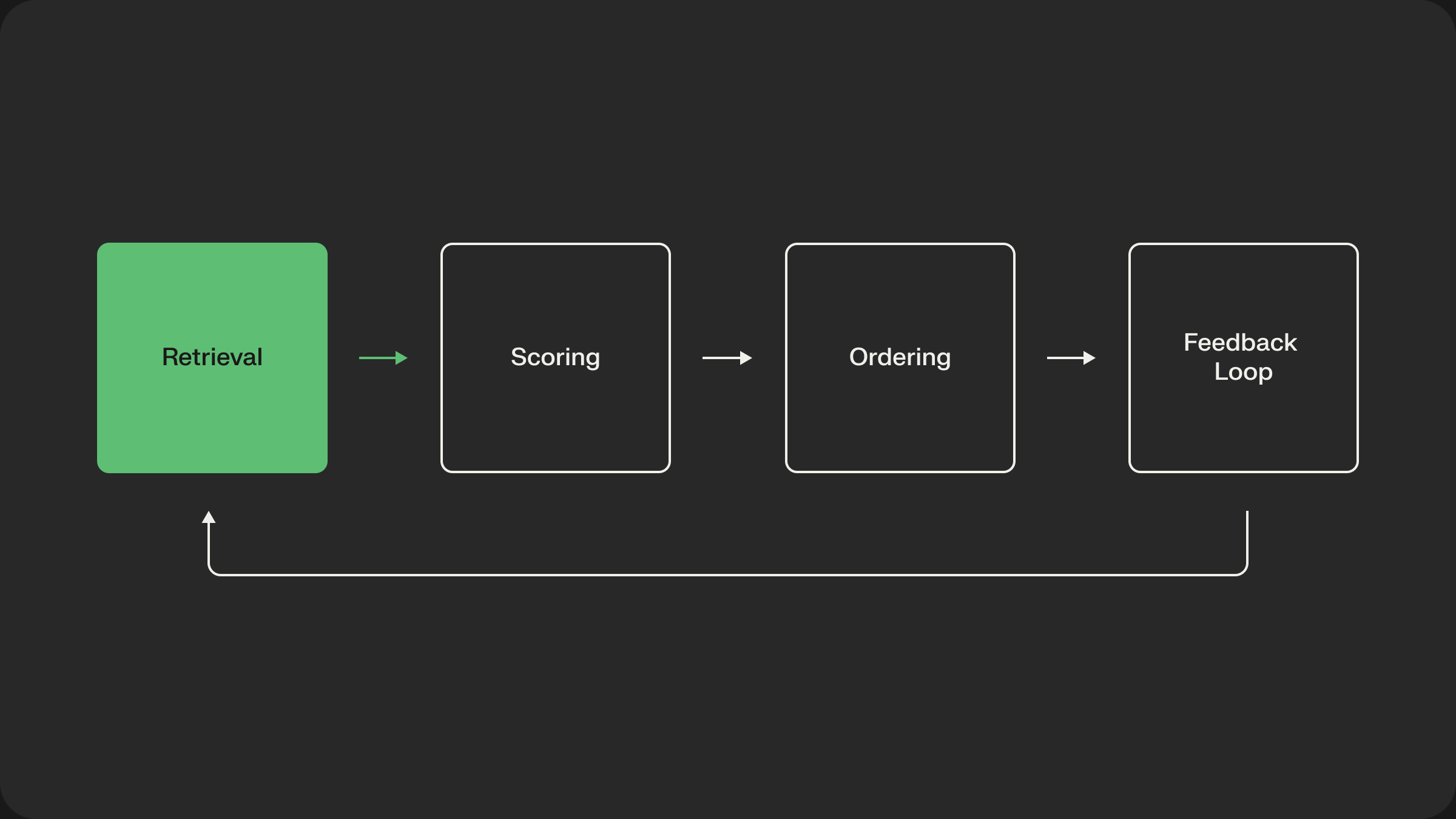
The retrieval stage is a complete system in its own right, with a careful balance of offline preparation and online execution. It's an ensemble of different strategies—heuristics, memorization, and generalization—all working in parallel to produce a high-recall candidate set under strict latency constraints. It's the foundation upon which the entire relevance pipeline is built.

Now that we have our high-recall set of candidates, we can finally afford to get precise. In the next post, we'll dive into the Scoring Stage, where we'll use powerful deep learning models like DLRMs and Transformers to assign exact relevance scores to each of these candidates.