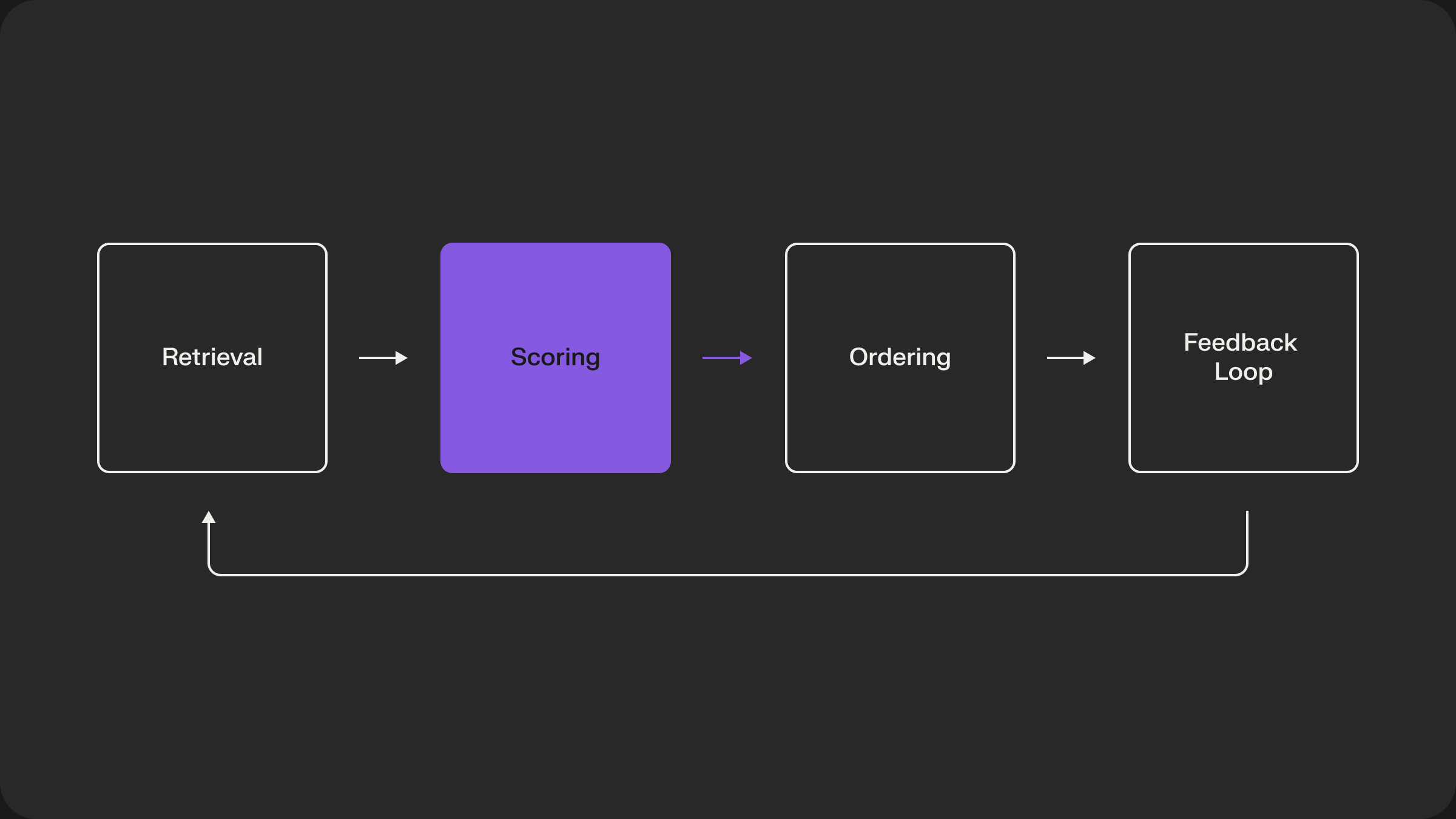
The Scoring Stage: The Art of Pointwise Prediction

That Retrieval Stage was about casting a wide net to ensure we didn't miss potential gems. The Scoring Stage is where we get out the jeweler's loupe. Its job is to apply a much more powerful, computationally expensive model to this smaller set of candidates to calculate precise, multi-objective scores for each one. This is where we shift our focus from recall to precision.

This stage is a higher-fidelity approximation of our "perfect scorer" function. We can afford to use richer features and more complex models because we are only dealing with a thousand items, not billions.

The Pointwise Scoring Task

The fundamental task of the scoring stage is pointwise prediction. For each candidate item, we want to answer one or more questions independently:

• What is the probability this user will click on this item? (p(click))
• What is the probability this user will purchase this item? (p(purchase))
• What is the predicted watch time for this video? (predicted_watch_time)

Each (user, item, context) triplet is scored in isolation. The model doesn't know about the other candidates in the set; its only job is to produce the best possible score for the one item it's looking at.

The Real Engine: A Deep Dive into Feature Engineering

Machine learning models are just sophisticated pattern matchers. The quality of their predictions is fundamentally limited by the quality of the signals we provide them. In recommendation systems, this process of creating signals is called feature engineering, and it is arguably more important than the choice of model architecture itself.

Feature Categories

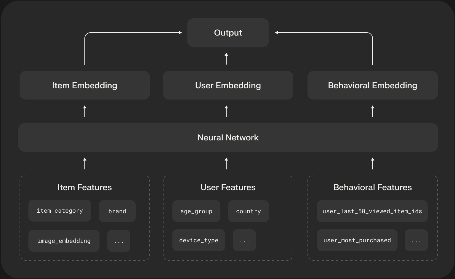
The features that power a scoring model can be broken down into a few key categories:

1. Item Features: Static or slowly changing metadata about the item being scored. These are typically easy to source and serve.
   
   • Examples: item_category, price, brand, textual_description, image_embedding.
2. User & Context Features: Information about the user and the context of their request.
   
   • Examples: User demographics (country, age_group), user's device (device_type), time of the request (time_of_day, day_of_week).
3. Behavioral (Historical) Features: These are the most powerful and predictive features. They summarize a user's past interactions to model their current intent.
   
   • Aggregated Features:
   • Features computed over a long time window, like a user's historical click-through rate on a specific category (user_ctr_on_electronics_30d) or their favorite brand (user_most_purchased_brand).
   • Sequence Features:
   • A raw, ordered list of a user's most recent interactions, such as user_last_50_viewed_item_ids. These are crucial for modern sequential models.
   • Negative Interactions: A user's history of what they've been shown but have not clicked on is a powerful negative signal that helps the model learn what the user dislikes.

The Engineering Backbone: The Feature Store

Managing these features at scale is a massive engineering challenge. This is where a Feature Store becomes essential. A feature store is a centralized system that manages the entire lifecycle of features, from generation to serving.

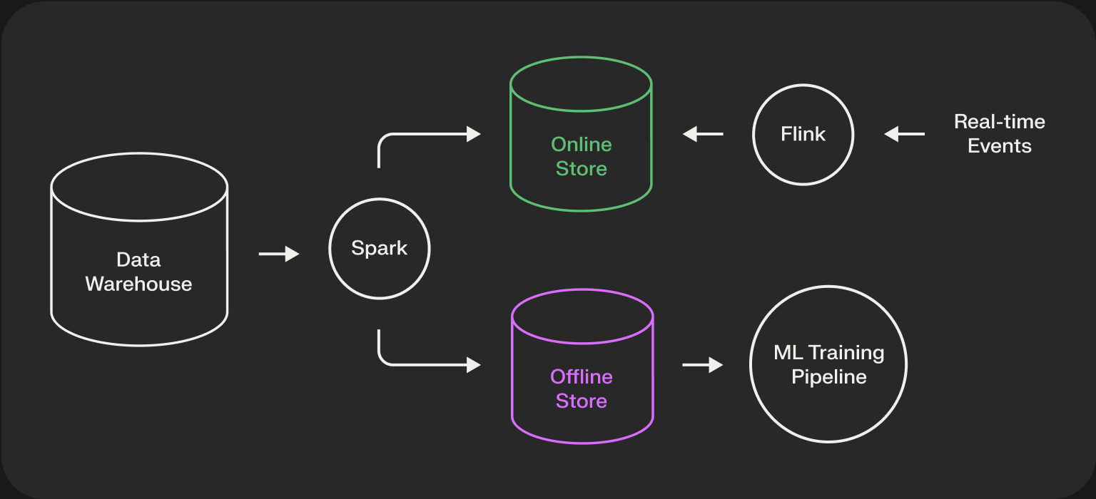
Its key responsibility is to solve the online/offline skew problem. It does this by providing two interfaces to the same feature data:

• Offline Store: A historical, high-throughput data store (e.g., a data lake or warehouse like S3, BigQuery). This is used to generate large datasets for model training.
• Online Store: A low-latency, real-time key-value store (e.g., Redis, DynamoDB). This is used by the online recommender system to fetch fresh features for inference in milliseconds.

By using the same feature generation logic for both stores, a feature store guarantees that the data the model was trained on is consistent with the data it sees in production.

The Foundational Approach: Feature-Based Models in PyTorch

Now that we understand where our features come from, let's build a model that can consume them. We will use PyTorch to build a simple but effective CTR prediction model that incorporates numerical, categorical, and multi-valued behavioral features.

This model demonstrates:

1. Using nn.Embedding for single categorical features like item_category.
2. Using nn.EmbeddingBag to efficiently process a list of recent interactions (user_last_n_item_ids) by averaging their embeddings.
3. Combining all feature representations for a final prediction.

1 import torch
2 import torch.nn as nn
3 import numpy as np
4 
5 # --- Feature Definitions & Vocabulary ---
6 VOCAB_SIZES = {'item_id': 1000, 'item_category': 20, 'device_type': 5}
7 NUM_DENSE_FEATURES = 1  # e.g., user_age_scaled
8 
9 # --- Offline Training ---
10 class SimpleScoringModel(nn.Module):
11     def __init__(self, vocab_sizes, embedding_dim=16, last_n=10):
12         """A simple but powerful feature-based model in PyTorch."""
13         super().__init__()
14 
15         # --- Embedding Layers for Categorical Features ---
16         self.item_embedding = nn.Embedding(vocab_sizes['item_id'], embedding_dim)
17         self.category_embedding = nn.Embedding(vocab_sizes['item_category'], embedding_dim)
18         self.device_embedding = nn.Embedding(vocab_sizes['device_type'], embedding_dim)
19 
20         # --- EmbeddingBag for Behavioral Features ---
21         self.history_embedding_bag = nn.EmbeddingBag(
22             vocab_sizes['item_id'],
23             embedding_dim,
24             mode='mean'  # Average the embeddings of the last N items
25         )
26 
27         # --- Final Classifier ---
28         input_dim = NUM_DENSE_FEATURES + (embedding_dim * 4)
29         self.classifier = nn.Sequential(
30             nn.Linear(input_dim, 64),
31             nn.ReLU(),
32             nn.Linear(64, 1)  # Output single logit for binary classification
33         )
34 
35     def forward(self, dense_features, categorical_features, history_features):
36         """Forward pass of the model."""
37         item_emb = self.item_embedding(categorical_features['item_id'])
38         cat_emb = self.category_embedding(categorical_features['item_category'])
39         dev_emb = self.device_embedding(categorical_features['device_type'])
40         history_emb = self.history_embedding_bag(history_features)
41 
42         combined_features = torch.cat([
43             dense_features,
44             item_emb,
45             cat_emb,
46             dev_emb,
47             history_emb
48         ], dim=1)
49 
50         logit = self.classifier(combined_features)
51         return logit

Beyond Clicks: Multi-Objective Optimization and Composed Value Models

A recommender trained solely to optimize for clicks will inevitably learn to serve clickbait. A modern recommender must optimize for a multi-objective value function that aligns with the long-term health of the business and user satisfaction.

A powerful and intuitive approach is to model the user's conversion funnel explicitly. Let's say our goal is to predict the probability of a purchase. We can decompose this using the chain rule of probability:

p(Purchase) = p(Click) * p(Purchase | Click)

This is an incredibly useful modeling strategy. We train two separate models (or two heads of the same model):

1. A CTR model (p(Click)) is trained on all impressions.
2. A Post-Click CVR model (p(Purchase | Click)) is trained only on items that were clicked.

This correctly handles the severe selection bias in the data and allows each model to learn from a cleaner distribution.

Once our model outputs these multiple predictions, the final step is to combine them into a single score that the ordering stage can use. This is where machine learning meets business logic. The final score is a composed value function.

• E-commerce:
• score = p(click) * p(purchase | click) * item_price
• Video Recommendations:
• score = p(click) * predicted_watch_time
• Social Media:
• score = w_like * p(like) + w_comment * p(comment)

This composed score is the final output of the Scoring Stage, ready to be passed to the Ordering Stage for the last mile of ranking.

Online: Real-Time Feature Hydration and Inference

Once the models are trained offline, they are deployed to a serving environment. When a request comes in with its ~1000 candidate IDs, the online system has to assemble the feature vectors for each one and run inference, all within a few dozen milliseconds. This process is often called feature hydration. 

The online scoring path for a single candidate looks like this: 

1. Fetch Static/Pre-computed Features: Look up item metadata (e.g., category, brand) from a fast key-value store like Redis. These features are static and shared by all users.
2. Fetch Real-time Features: This is the most latency-sensitive step. Look up fresh user features (e.g., items interacted with in the last 5 minutes) and context features (e.g., device type) from a very low-latency feature store.
3. Assemble the Feature Vector: Combine the static, real-time, user, and context features into the exact tensor format that the trained model expects.
4. Model Inference: Batch the 1000 assembled feature vectors and send them to the deployed scoring model (often served on a GPU or other accelerator) for prediction. The model returns a list of scores.

1 def score_candidates(candidate_ids, user_id, context, model, feature_store):
2     """ Hydrates features and scores a batch of candidates. """
3     feature_vectors = []
4     # Fetch real-time user features once
5     user_features = feature_store.get_user_features(user_id)
6     for item_id in candidate_ids:
7         # 1. Fetch static item features
8         item_features = feature_store.get_item_features(item_id)
9 
10         # 2. Assemble the full feature vector
11         # This must match the format the model was trained on.
12         feature_vector = assemble_feature_vector(
13             user_features,
14             item_features,
15             context
16         )
17         feature_vectors.append(feature_vector)
18 
19     # 3. Run batched model inference
20     # In a real system, this would involve converting to tensors
21     # and sending to a model serving endpoint.
22     scores = model.predict(feature_vectors)
23 
24     # Return a list of (item_id, score) tuples
25     return list(zip(candidate_ids, scores))

Conclusion

The Scoring Stage is the analytical heart of the recommender system. It's powered by rich, carefully engineered features and flexible models that can predict multiple, business-aligned objectives. We've taken a large, unfiltered set of candidates and attached precise, meaningful scores to each one.

But a list of items with independent scores is still not a final product. How do we blend candidates from different sources? How do we ensure the final page is diverse and not repetitive?

In our next post, we'll dive into the Ordering Stage, where we transform this scored list into a polished, fully-constructed user experience.