
If someone had previously watched movies like: Avengers, Top Gun, and Star Wars, they’re probably going to enjoy the movies on the first list more. We assume this because our prior understanding of the movies (e.g. genre, cast, set) allows us to evaluate which list is most similar to the historical watch list. However, imagine you knew a majority of people that previously watched the same movies and happened to also enjoy the movies on the second recommendation list, you might conclude that the second recommendation list is actually more relevant. These two ways of deciding relevance are what recommendation systems aim to learn from your data [1].
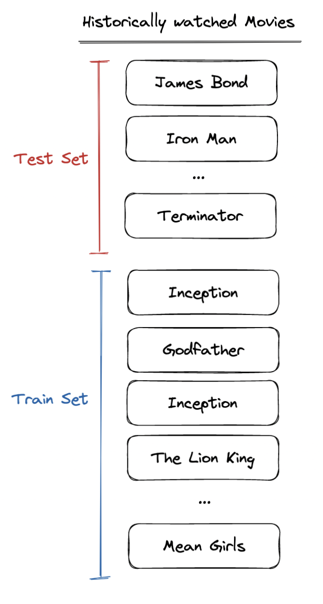
How can we objectively measure which recommendation algorithm is best to serve to your user? One way to evaluate the algorithms offline [2] is through a process called ”cross-validation”, where the historical watch list (i.e. the list of relevant items) is chronologically split [3] into train and test sets. The recommendation algorithms are trained on the train set and performance metrics are evaluated on the test set. These performance metrics can then be used to objectively measure which algorithm is more relevant.
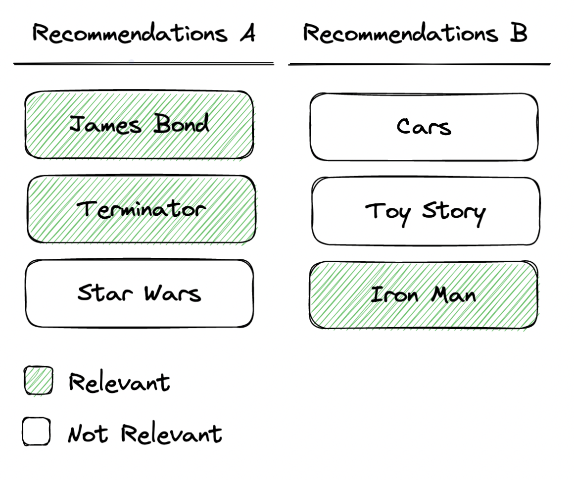
Continuing on with the example, let’s assume that the test set for the user in question contains: The Terminator, James Bond, Iron Man, and 3 other unrelated movies. We can measure performance by comparing the matches between the evaluation set and both recommendation lists. Two classic metrics that are used are: Precision@k and Recall@k.
Precision@k
**Precision@k measures the proportion of relevant recommended items in a recommendation list of size k. For the first recommendation list (The Terminator, James Bond, and Love Actually), we can see that there are 2 matches out of the 3 items. For the second list, there is 1 matches out of the 3 items. Therefore:
- Algorithm A, Precision@3 = 2/3 = 0.666
- Algorithm B, Precision@3 = 1/3 = 0.333
 Precision@k = (number of relevant recommended k items) / kA: Precision@3 = 2/3, B: Precision@3 = 1/3
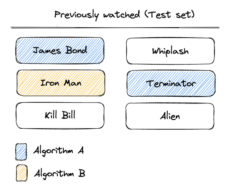
Recall@kThe other way we can define matches is based on the proportion of relevant recommended items (in the recommendation list of size k) and the total number of relevant items. This metric is called recall@k. For example, the user has watched 6 movies, and in the first recommendation list, 2 of them are relevant. In the second list, 1 of them are relevant. Therefore:
- Algorithm A, Recall@3 = 2/6 = 0.333
- Algorithm B, Recall@3 = 1/6 = 0.166
 Recall@k = (number of relevant recommended k items) / (total relevant items)A: Recall@3 = 2/6, B: Recall@3 = 1/6
In our example, algorithm A is more relevant because it has higher Recall@k and Precision@k. We didn’t really need to compute both to understand this, if you look closely you’ll notice that if one of these metrics is comparatively higher to another algorithm then the other metric will be equal or higher too. Regardless, it’s typically worthwhile looking at both of these metrics for the interpretable understanding they provide.
Precision@k gives us an interpretable understanding of how many items are actually relevant in the final k recommendations we show to a user. If you are confident on your choice of k, it typically maps to the final recommendation well and it’s easy to communicate. The problem is that it’s strongly influenced by how many relevant items the user has. For example, imagine our user only watched 2 relevant items, the maximum Precision@3 they could achieve with a perfect recommendation system is capped at: Precision@3 = 2/3 = 0.666. This causes issues when averaging the result across multiple users.
The best of both worlds: R-PrecisionA metric that solves these issues with Precision is called *R-Precision.*It adjusts k to the length of the user’s relevant items. For our example in the last paragraph (where the user has only watched 2 movies), this means that we have R-Precision=2/2=1, for a perfect recommendation system, which is what we’d expect.
R-Precision = (number of relevant recommended top-r items) / r Where r is the total number of relevant items.
Note that when r = k, Precision@k, Recall@k and R-Precision are all equal.
When we have a fixed budget of recommendations k, like in the example we’re running with, you probably want to cap k. This capped metric, R-Precision@k, can be thought of as Recall@r when the number of relevant items is less than k and Precision@k when it’s greater than k. It gives us a best of both worlds of the two metrics and averages well across users.
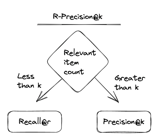 R-Precision@k = (number of relevant recommended top-s items) / sWhere s = min(k, r)
What’s next The metrics we’ve gone over today: Precision@k, Recall@k, R-Precision, are classic ways of evaluating the accuracy of two unordered sets of recommendations with fixed k. However, ranking order can be crucial to evaluate the quality of recommendations to your users, particularly for recommendation use-cases where there’s minimal surface area to show your recommendations and every rank position matters. Alternate objectives such a diversity and bias also need to be considered beyond the relevance accuracy metrics we talked about today. Finally, all these metrics are great for offline evaluation with cross-validation but it’s important not to forget about online evaluation — that is, measuring the results after you’ve started surfacing the recommendations directly to users. In the next posts, we’ll discuss each of these recommendation evaluation topics. Stay tuned!
Written in collaboration with Nina Shenker-Tauris.
Footer:
-
The first method, where similarity of content is used to determine what’s relevant is called “Content-based filtering”. The second method, where the people’s shared interests are used to determine what’s most relevant is called “Collaborative filtering”.
-
As opposed to online, where we surface the recommendations directly to the users
-
We use a chronological split to ensure that information about historic data isn’t leaked in the test set.
-
Note we define all metrics for a specific user but in practice they’re often defined as averages across every user in the test set.
See Shaped in action
Talk to an engineer about your specific use case — search, recommendations, or feed ranking.