
As AI continues to permeate throughout the tech landscape, companies now face an approaching reality where nearly all of their decisions are in part fuelled by the conclusions machine learning models discover from analysing data from every facet of their business. From social media interactions to freeform reviews of a product within a market place, businesses now face the challenge of gaining key insights into the minds of their customers from the data that is generated from their online ecosystems. For numerical data, this process is relatively straightforward using traditional Data Science methods, but what of other types of data that cannot be treated as such?
Enter Embeddings, the process of transforming non-numerical data into a representative numerical vector space that can be appropriately used as inputs to machine learning algorithms. In this blog, we will discuss the core of what embeddings actually are, how they are generated, and the issues and decisions faced when attempting to convert unstructured data into vectors that allow AI to do its magic as intended.
What really are Embeddings?
At its core, the concept of embedding a piece of data revolves around a mathematical transformation that projects the data into a n-dimensional space. The aim of this transformation is to reduce the dimensionality of the original data whilst preserving the maximum amount of information contained within, so that similar data points are located together when embedded into n-dimensional space. More precisely, consider a dataset Xwith ndimensions and a function f with mdimensions such that:
fis injective, where each individual point xin X corresponds to an individual point f( x) in f( X). This is commonly known as the one-to-one property.
f is structure preserving, where the result of mathematical operations in X are preserved in f( X). For example, fwould be structure preserving of multiplication if for any two points in X*:*
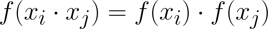
If a function fsatisfies both of these qualities above, then it is said to be an embedding function on X
For real world data that is complicated and unstructured, this function f wouldn’t be analytical in nature, meaning that we couldn’t write it down as a simple equation. Instead, the algorithm that represents f is an embedding algorithm if it transforms our data into vector space whilst obeying these qualities. Despite all the fancy symbols and terminology above, the process at its core is really quite simple. We are taking non- numerical data, and converting it into vectors so that two pieces of original data that are similar to start with are numerically similar once embedded.
Although this idea of turning words, images, videos, etc into numerical vectors does seem like a cool trick, what is the point of all this? The answer to this lies in the second condition of an embedding algorithm, the structure preservingquality. Let’s consider two of my favourite shows at the moment which I have been binge watching at a rather unhealthy pace, Succession& Billions:

As a side note, if you haven’t watched either of these two shows, do yourself a favour. Brilliant acting, brilliant casts. Succession centres around the internal power struggle of the children of a media mogul for control of his empire, whilst Billions tells the story of a cat and mouse game between a hedge fund manager and a US attorney. Although these shows have their slight differences, they are often compared to each other as the modern seminal pieces of TV in what could be called the Financial Drama genre.
Anybody who watches a couple of episodes of each could easily see the link between the two, and identify the semantic similarities. But how in the world would a machine learning algorithm be able to do that? This is where embeddings become essential in today’s AI. If we were able to embed the script of the two shows into a n-dimensional vector space, the structure preserving quality of the embedding algorithm would map the two into locations that are geometrically close together. This distance in vector space is how the computer understands and infers semantics:
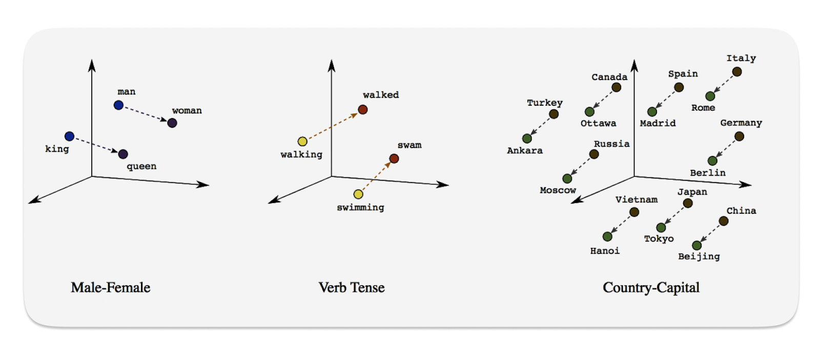 Note that embedding architectures preserve the concept of semantic similarity by inferring it as the distance between two points in vector space.
So how do we create Embeddings?
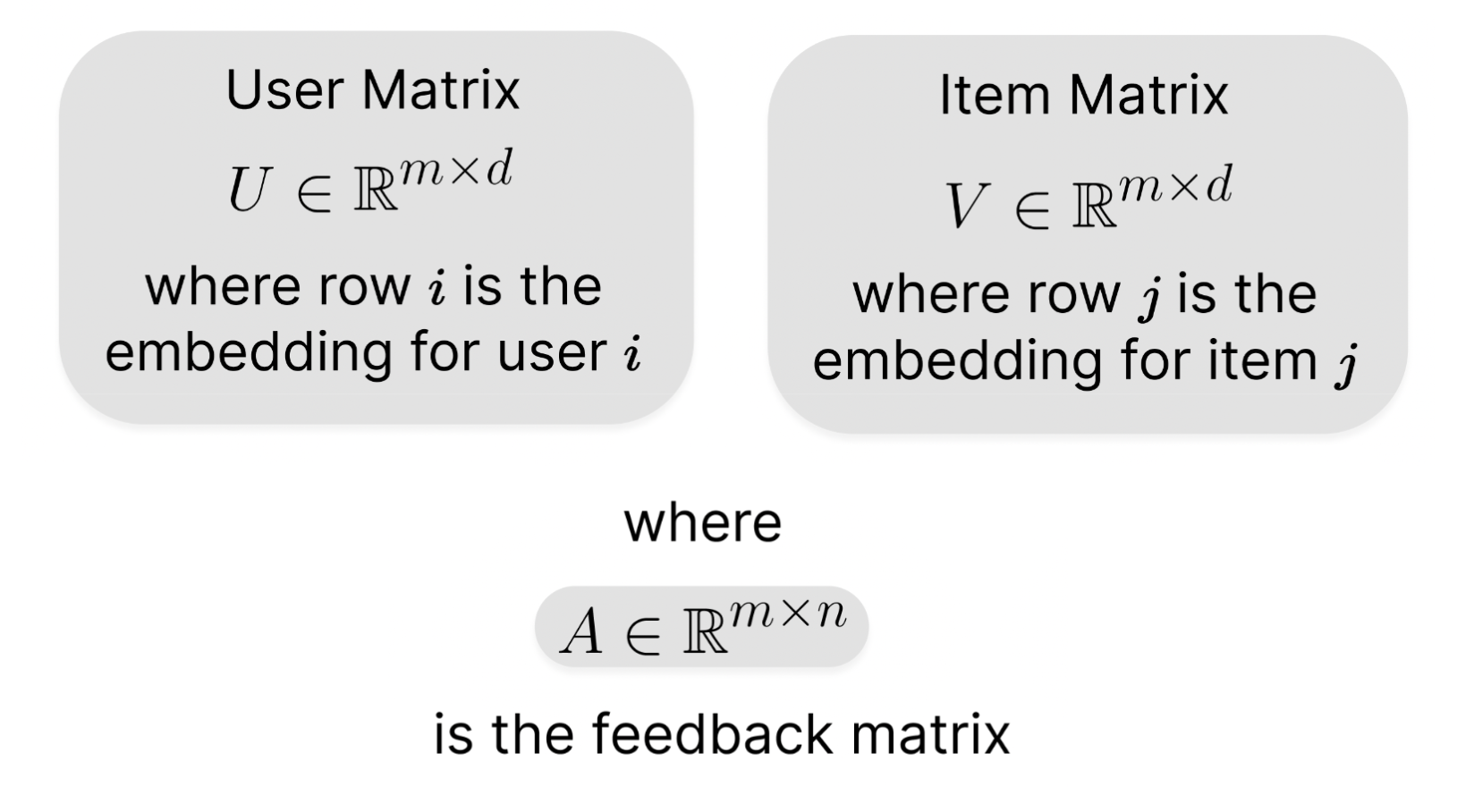
Let’s say we want to build a recommendation system for showing listeners albums they are interested in. We can achieve something like this (as well as a lot of tasks analogous to this) by using Matrix Factorization, one of the more commonly widespread embedding methodologies. We begin by defining the following:
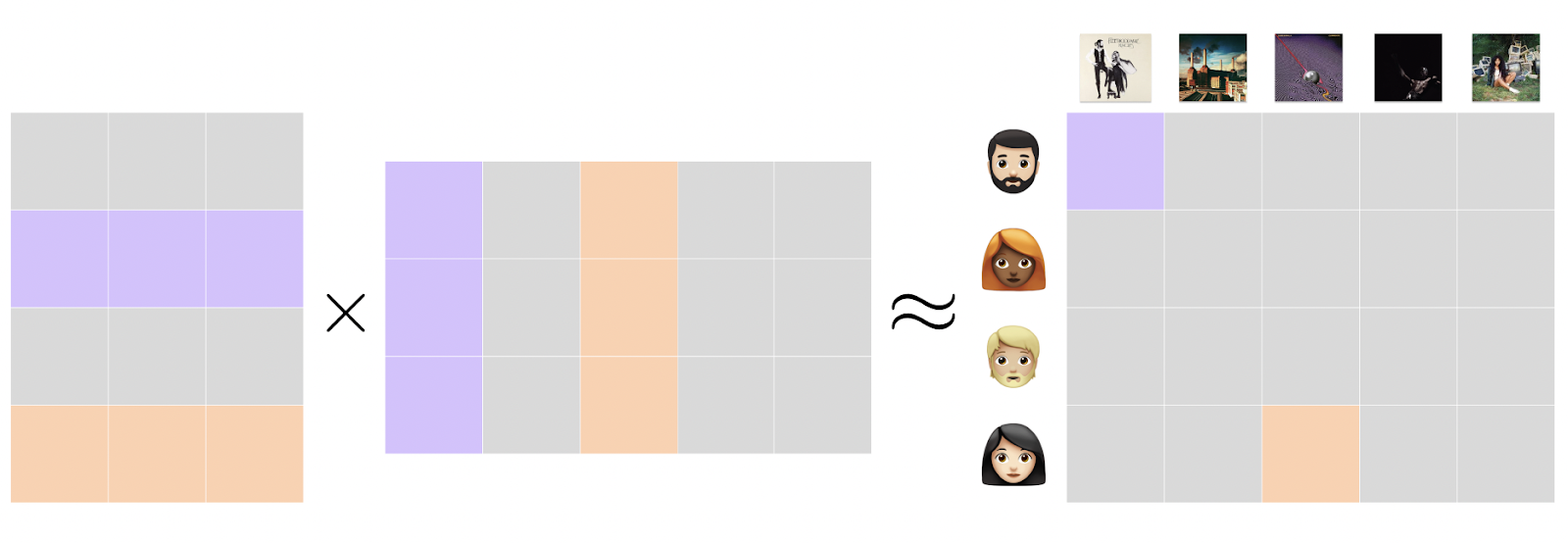 Each user row and item collumn is used to generate the feedback cell for a given interaction event. These values are what we are trying to minimise in order to create our optimal interaction embedding space!
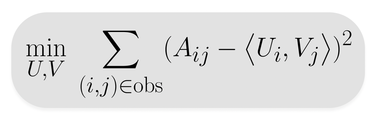
The embeddings are learned so that the matrix product of the user and item matrices are an accurate estimation of the feedback matrix. Each point in this matrix is the dot product of the of the embeddings of the ith user and jth item. Now, how do we go about finding the values for U and V such that this condition holds? Firstly, we have to choose and construct an Objective Function to minimize. To do this, we consider minimizing the approximation errors for each entry:
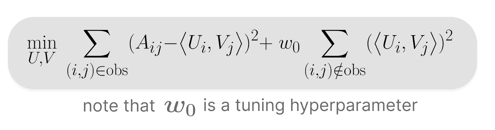
Now, in order to account for potential unobserved entries within the value of UVT, we need to split this objective function in two, one part that represents the sum over all observed entries and the other that represents the sum over all unobserved entries:
This adjusted objective function has an analytical solution in vector space, which can be calculated using the Gradient Descentalgorithm, a common foundation for most machine learning models. Without going to deep into this method, it is an iterative approach to finding the local minimum of a multidimensional function where we:
- Take a Starting Point in space
- Calculate the Gradient at that point (i.e How steep the curve is and in what direction)
- We crawl in the opposite direction of this gradient to a new point
- Repeat step 2 at this new point
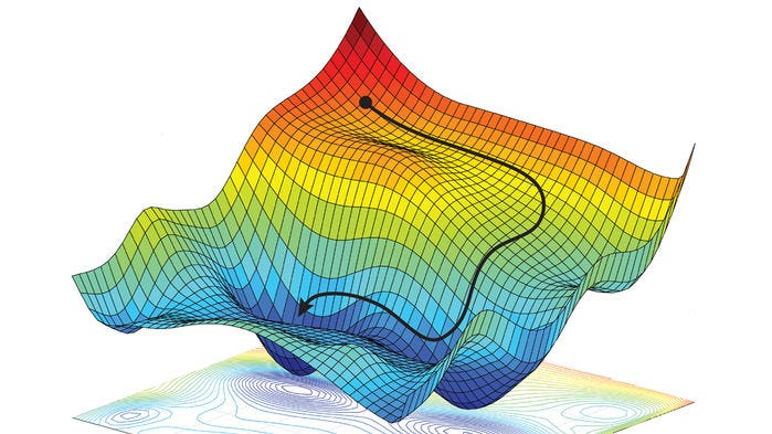 This iterative process is at the heart of all ML methods & how they arrive at their optimal hyperparameters
Once we have solved this equation, we now have embeddings! The user and item matrices have been trained so that they are as close to the feedback matrix, which happens to be created from past historical data. Now that the features have been embedded, the task of defining similarity between these features arises. This is where the concept of vector space distance comes into play. The two main ways of measuring similarity for use cases such as these are Euclidean Distanceand Cosine Similarity:
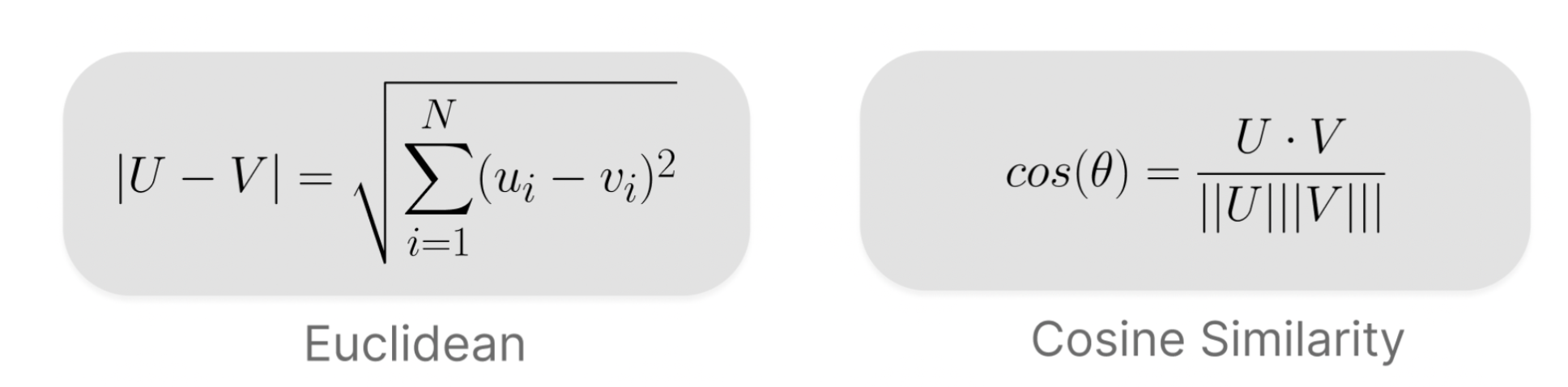
Euclidean Distance measures the geometric distance between two vectors, a simple extension of Pythagoras’ Theorem. Cosine similarity on the other hand, measures the angular distance between two vectors, taking in account their angular separation and normalising for their length. Other less traditional measures of vector distance are out there, but these two are the most commonly used for the majority of machine learning models. For the case of a recommender system, we want our measured similarity not to take in account the varying dimensionality of any two embedded vectors. Since we are operating with two key types of vectors with different structure, we want to be concerned with the direction of our vectors rather than their geometric length. This is where cosine similarity is an appropriate choice.
Note that although this methodology is with the use case of recommendation systems in mind, all other embedding processes consist of the construction of analogous minimisation problems in tandem with a choice of similarity measurement. These two parts are at the core of embeddings, and are in many ways, practical extensions to the two mathematical properties of a base level embedding function in pure mathematics mentioned above. By enforcing both of these concepts, embeddings opens the doorway between tangible real world data (that is often messy and semantic) and the mathematical intelligence of modern machine learning. It is a lot more than just a neat maths trick, it is the very thing that allows current AI to translate both our digital and physical worlds into something it can actionably process.
This transformation from unstructured and often overwhelming data into vector embeddings allows machine learning algorithms to uncover patterns and relationships within your data that are quite simply invisible to the human eye. The majority of data that is truly useful for users, companies and businesses is of such high dimensional complexity that we simply can’t infer the true context of our data points through conventional data science. Whether it’s linking the thematic elements of two tv shows, or tailoring recommendations of products to individual users, passing unstructured and multimodal data through modern vector embedding algorithms unlocks the door for AI to semantically reason in a manner adjacent to ourselves, and harness its computational superiority to us to generate insights that would have otherwise never been noticed.
See Shaped in action
Talk to an engineer about your specific use case — search, recommendations, or feed ranking.