But in production Recommendation Systems (RecSys) and Search (IR), tokenization is a different beast entirely.
In RecSys, our “tokens” aren’t words, they are User IDs and Item IDs. Unlike the English language, this vocabulary never stops growing. Every time a new user signs up or a new product is listed, the “vocabulary” expands. We aren’t dealing with 50,000 tokens; we are dealing with 10 million, 100 million, or even billions of unique entities.
At Shaped, we’ve spent the last month deep in the trenches of this problem. We realized that while the industry is currently obsessed with LLM context windows, the most significant bottleneck in production RecSys remains the Distributed Bottleneck: the engineering debt incurred when you try to map a chaotic, high-cardinality world into a rigid, stateful embedding table.
Tokenizer vs Embedding
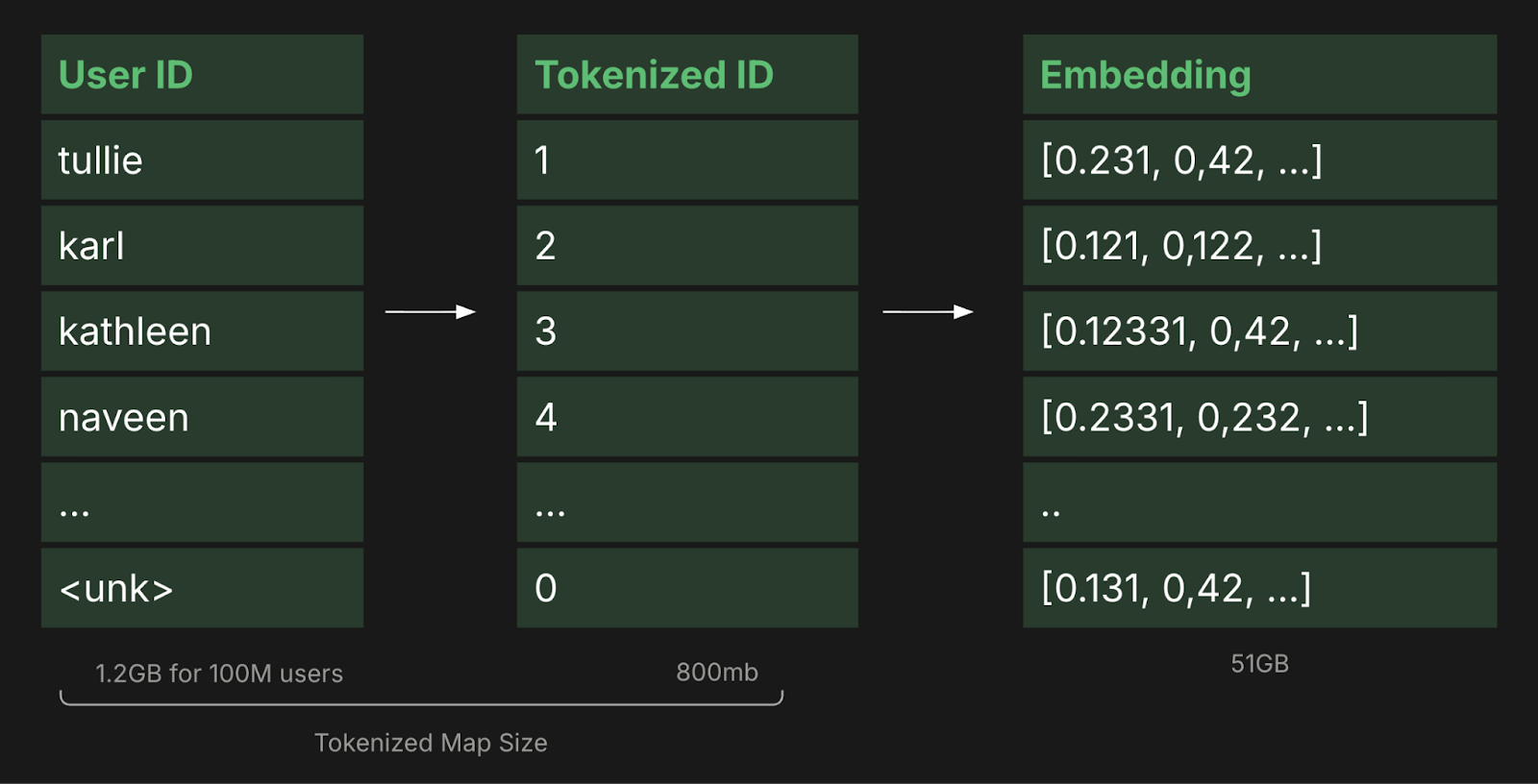
When we talk about “the scale problem,” we are actually fighting a two-headed monster: the ID Map in System RAM and the Embedding Table in VRAM.
In a standard “naive” RecSys architecture, your system is split into two expensive stages:
- The Tokenizer (System RAM): This is a massive hash map (often a Redis instance or a distributed std::unordered_map) that maps a string (e.g., user_8f21) to an integer index (e.g., 402,121). At 100M IDs, just the keys and values of this map can consume 10GB+ of RAM. If you are running a distributed training cluster with 64 workers, keeping every worker’s ID map in sync becomes a distributed systems nightmare.
- The Embedding Layer (VRAM): This is the actual weight matrix where row 402,121 contains the 128-float vector for that user. These weights must live on the GPU for the model to compute gradients efficiently. A 100M-ID table at 128-dimensions requires ~50GB of VRAM. Add an optimizer like Adam (which tracks two moments per weight), and you’re at 150GB+.
You hit this wall much sooner than you think. Even at 10 million IDs, your training setup is already too fat for a single consumer GPU, and your data pipeline is likely lagging as it tries to coordinate ID mappings across workers. You find yourself sharding models and building complex token maps not because your neural network is complex, but because your “dictionary” is unmanageable.
The Distributed Bottleneck
The real pain of “standard” tokenization isn’t just memory; it’s the infrastructure required to keep the system coherent:
- Synchronization Lag: Every time a new ID is created, every training worker and inference node must “agree” on its new index. If an inference node is even a few seconds out of sync with the latest ID mapping, it will return garbage for new users, exactly when first impressions matter most.
- The “Cold Start” Death Spiral: Standard tokenization treats every ID as an island. If the model hasn’t seen ID_A before, it falls back to a generic
<UNK>(Unknown) token. You throw away the opportunity to learn that ID_A might be mathematically similar to ID_B based on its metadata.
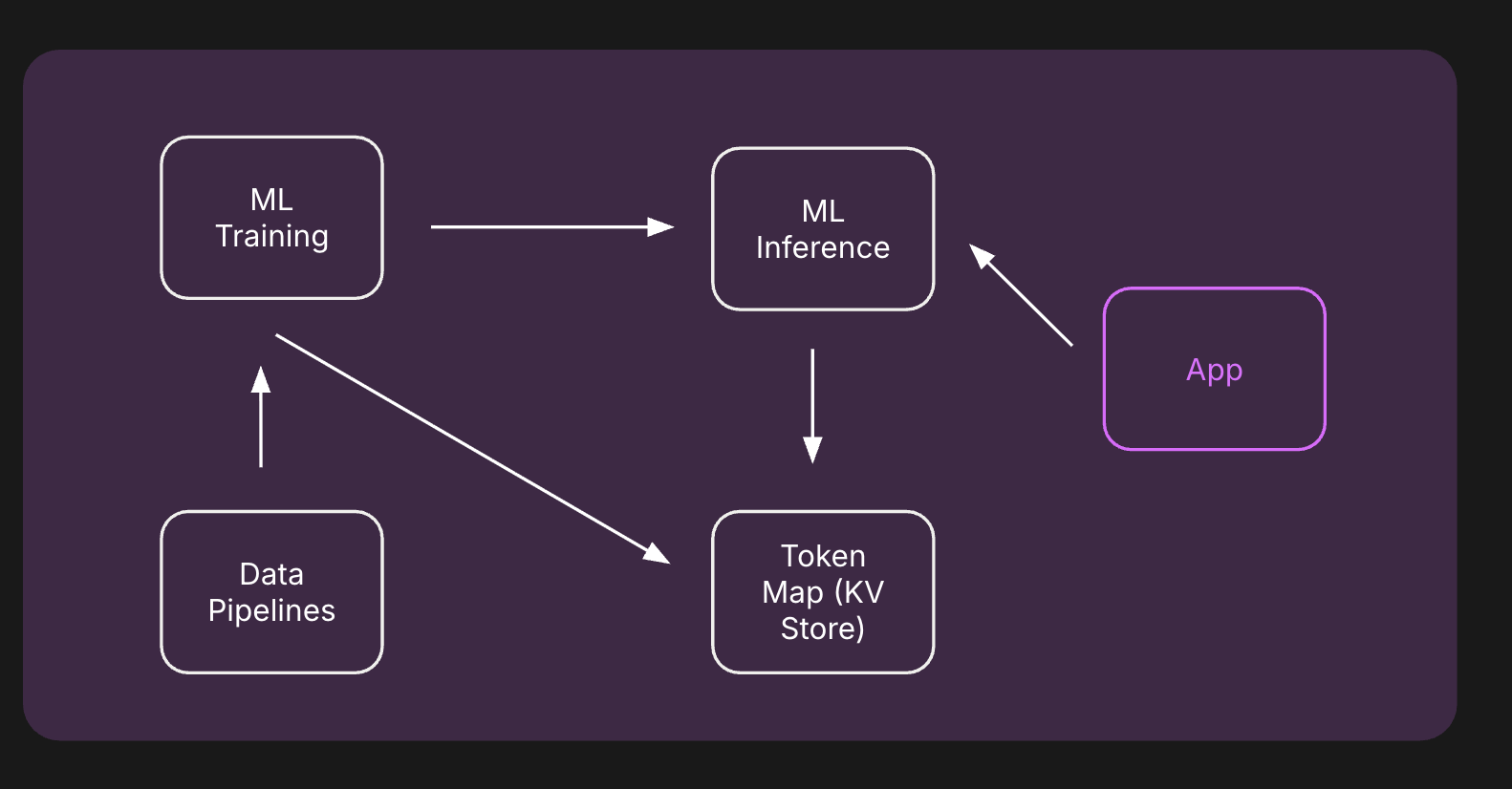
Moving from “Lookup” to “Compute”
The challenge we’ve been solving at Shaped is how to move away from Stateful Lookups (mapping an ID to a row in a table) toward Stateless Factorization (calculating a representation directly from the ID).
This shift turns RecSys from a database problem into a math problem. By replacing the lookup dictionary with a deterministic mathematical function, you can:
- Delete the RAM-based ID Map entirely.
- Compress the VRAM-based Embedding Table into a fraction of its original size.
- Improve performance on the “tail” of your data where IDs are rare or new.
In the next sections, we’ll dive into the academic evolution of this problem, from the “Hashing Trick” to the Cuckoo Hashing strategies popularized by TikTok’s Monolith paper, and the specific architecture we built at Shaped to solve these bottlenecks.
The Evolution of Dynamic Representation
How do you represent a billion IDs in a way that doesn’t melt your infrastructure? This question has been the subject of a decade-long arms race in industry research. Each evolution attempts to solve the same fundamental trade-off: How much collision (error) are we willing to accept in exchange for a smaller memory footprint?
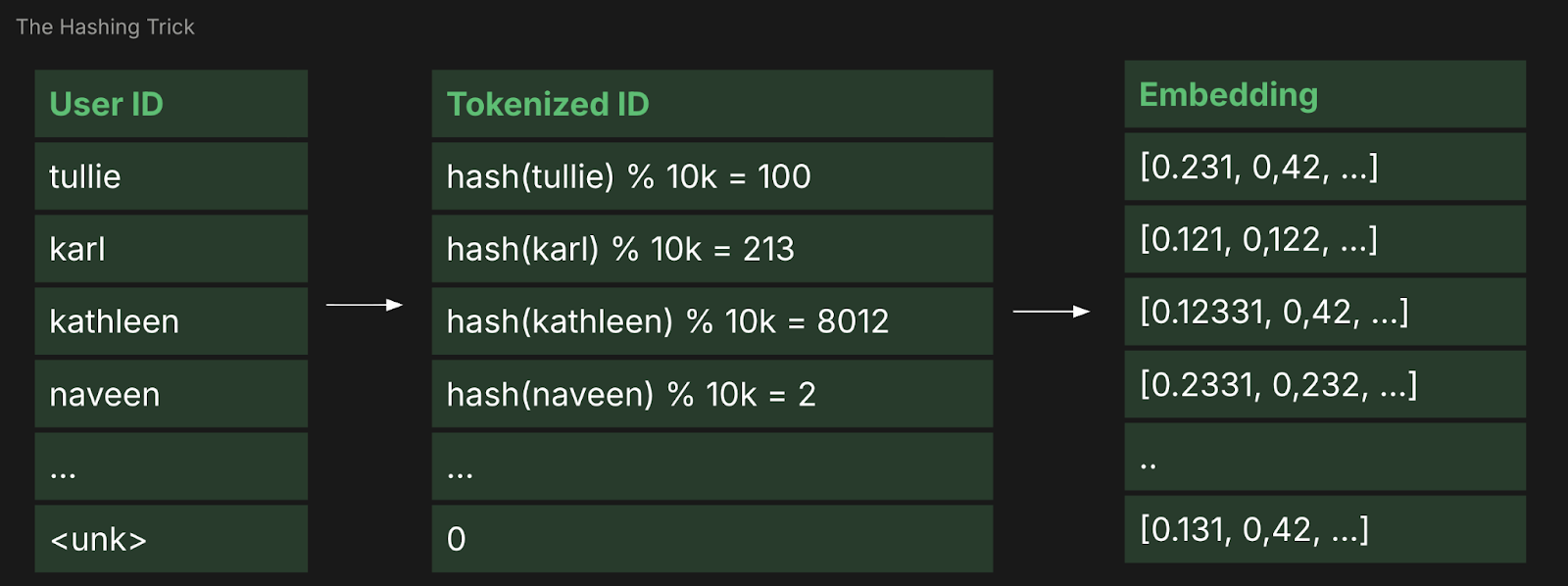
1. The Hashing Trick (2009)
The oldest and simplest approach to stateless tokenization is the “hashing trick,” popularized by the Vowpal Wabbit project.
Instead of a lookup table, you simply take an ID, run it through a hash function, and apply a modulo operation: index = hash(ID) % TableSize.
- The System Win: It is completely stateless. You don’t need a token map. Any worker can calculate the index for any ID.
- The ML Failure: Collision Pollution. If User_A (a bot with 10k clicks) and User_B (a new, high-value customer) both hash to the same index, their gradients are summed together. The bot’s behavior will “pollute” the representation of the new user. At 10 million IDs and a 1-million-row table, the noise becomes catastrophic for the model’s performance on the “tail” of your data.
The Birthday Paradox
“How many people would you need in a room for it to be likely that two people share the same birthday?”
It’s easy to underestimate how quickly a hash table becomes “polluted.” If you have $N$ unique IDs and a hash table (or embedding table) of size $M$, the probability of at least one collision is $P \approx 1 - e^{-N^2 / 2M}$. (e.g. 1M users and a 10M hash table will have collision probability close to 1):
But in RecSys, we care about the Collision Density. If we have 100M items and a 10M-row embedding table, the number of IDs mapping to a single row follows a Poisson distribution with $\lambda = N/M = 10$.
- The Math: This means every row is trying to represent the average of 10 random ids simultaneously.
- The System Impact: When your model backpropagates, the gradient update for a “High-Value Buyer” is applied to the same weights as a “One-Time Bot.” This doesn’t just add noise; it creates gradient interference that prevents the model from ever converging on the “tail” of your distribution.
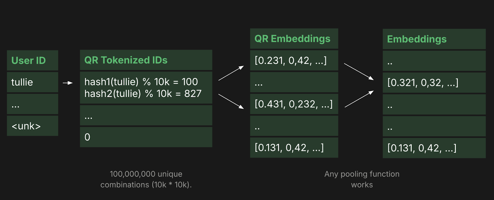
2. Meta’s QR Trick: The Power of $O(\sqrt{N})$ (2019)
In their paper “Compositional Embeddings Using Complementary Partitions,” Meta AI Research proposed a more elegant way to handle collisions. Instead of one large table, they use two smaller tables, let’s call them the Quotient table and the Remainder table.
To find the representation for an ID, you use two different hash functions:
- idx_1 = hash_1(ID) % 10,000
- idx_2 = hash_2(ID) % 10,000
The final embedding is a combination (e.g., addition or concatenation) of the vectors at these two indices.
- The Math: By using two tables of size 10,000, you only store 20,000 vectors, but you create an “effective” address space of $10,000 \times 10,000 = 100,000,000$ unique combinations.
- The Result: It dramatically reduces the probability that two IDs will share the exact same representation, all while keeping the memory footprint at $O(\sqrt
{N})$.
Collision Likelihood
This is why the QR Trick (Meta) and Multi-Hashing are so powerful. If you use two independent hash functions and two tables of size $B$, you aren’t just doubling your capacity. You are expanding your Address Space exponentially.
The probability of two IDs sharing the exact same representation (colliding in both tables) drops to: $$P(\text{total collision}) \approx \left( 1 - e^{-N^2 / 2B} \right)^k$$ (where $k$ is the number of hash functions)
Example:
- Single Table: 20,000 rows. Capacity = 20,000.
- QR Factorization: Two tables of 10,000 rows. Effective Capacity = $10,000^2 = 100,000,000$.
By using just 100kb of memory, you’ve created a unique “address” for every person on Earth. At Shaped, we found that moving from a large single table to a multi-hash projection reduced our VRAM usage by 85% while actually increasing our Recall@K because we finally eliminated the “collision noise” for our tail items.
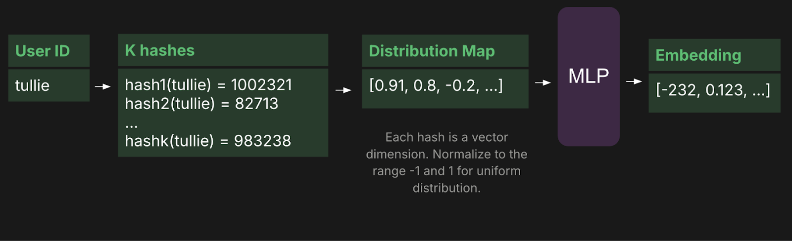
3. Google’s DHE: Moving from Table to Compute (2020)
Google Research took this to the extreme with “Learning to Embed Categorical Features without Embedding Tables” (Deep Hash Embedding). Their argument: why have a table at all?
DHE uses multiple hash functions to generate a “signature” vector for an ID (e.g., a 1024-dimensional vector of floats). This signature is then passed through a small, deep neural network (an MLP) that “decodes” the hash into a final embedding.
- The Systems Trade-off: You completely eliminate VRAM usage for the table. However, you pay for it in Compute. Every ID lookup now requires a forward pass through a small MLP. In high-throughput systems where you might be scoring 1,000 items per request, this latency adds up fast.
4. TikTok’s Monolith: The Collisionless Scaling King (2022)
Perhaps the most impressive production-scale solution comes from ByteDance (TikTok) in their paper “Monolith: Real-Time Recommendation System With Collisionless Embedding Tables.”
Unlike the “factorization” approaches above, Monolith doubles down on tables but solves the coordination and memory problems using two clever systems tricks:
- Cuckoo Hashing: They use Cuckoo Hash tables to manage the ID-to-embedding mapping. Cuckoo hashing allows for extremely high load factors (up to 95% table utilization) with nearly zero collisions, because it can “kick out” and re-locate items when a collision occurs.
- Expiring Embeddings: They realized that in RecSys, most IDs are ephemeral. Monolith implements a “TTL” (Time-to-Live) for every ID. If a user doesn’t visit for 30 days, their embedding is evicted from the table. This allows the system to handle an “infinite” stream of new IDs while keeping the memory footprint stable.
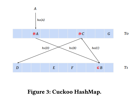
Why 95% Utilization Matters
Standard hash tables (like the ones used in Python or Java) start to fail when they are 50-60% full because of “clustering”, collisions start to chain together, and lookups slow down.
This is why TikTok’s Monolith uses Cuckoo Hashing. The math of Cuckoo Hashing allows you to reach >90% load factor without a performance hit.
- How it works: Every ID has two possible homes ($Hash_A$ and $Hash_B$). If $Hash_A$ is full, it kicks the existing ID to its own $Hash_B$ alternative.
- The System Result: You can pack twice as many User IDs into the same 80GB A100 GPU compared to a standard hash-based table.
5.Semantic IDs: The Generative Frontier (2023-2024)
While Hashing, QR, and DHE all try to compress IDs, they share a fundamental flaw: they are content-blind. In these systems, User_A and User_B are just random bits. If User_A is a new user who just signed up, the model has no choice but to treat them as a random cold-start entity.
In the last 18 months, spearheaded by researchers at Google, Meta, Netflix & Snapchat, there has been a shift toward Semantic Tokenization (or Semantic IDs).
Instead of assigning a random integer to a product or user, you use its features (titles, descriptions, categories, or images) to generate a “meaningful” ID.
- The Concept: You pass an item’s description through a pre-trained model (like BERT or a CLIP image encoder) and then use a technique like Product Quantization (PQ) or Hierarchical K-Means to turn that continuous embedding into a sequence of discrete tokens (e.g., Token_42-Token_129-Token_7).
- The System Win: Similar items naturally end up with similar “Semantic IDs.” If a brand-new “iPhone 15 Case” is listed, it will share tokens with other “iPhone Cases.” The model doesn’t have a cold-start problem because the “vocabulary” itself carries the meaning.
- The Challenge: This turns tokenization into a Generative Task. You aren’t just looking up an ID; you are running an inference pass on an encoder to decide what the ID is. This introduces a heavy latency penalty and a dependency on the stability of your encoder, if you upgrade your BERT model, all your “Semantic IDs” might shift, effectively lobotomizing your recommender.
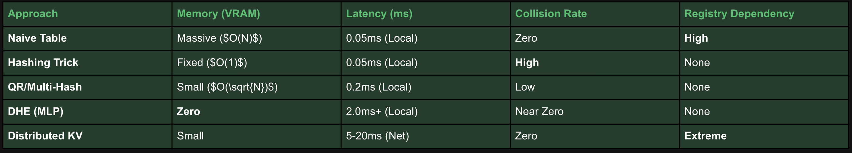 The Latency vs. Accuracy Trade-off
How We Tackled This Problem
These papers are brilliant, but they often assume you have the resources of a “Big Tech” firm: a dedicated parameter server team, custom C++ kernels, and petabytes of RAM.
At Shaped, our challenge was unique. Unlike TikTok or Meta, which manage a single, massive ID space, we are a multi-tenant platform. On any given day, we might be handling a customer with 10,000 items (where a simple dictionary is fine) alongside a customer with 500 million items (where a dictionary is a disaster).
We couldn’t build a custom tokenizer for every client and dataset. We needed a Single Universal Factorization Service that could adapt to any scale or model type.
The Shaped Strategy: A Multi-Model Decision Matrix
Handling IDs across a fleet of different model architectures taught us that a “one size fits all” tokenization strategy is a mistake. Instead, we built a logic flow that selects a strategy based on the model’s mathematical requirements:
1. The Small Scale (<100k IDs)
For smaller datasets, we use a standard dictionary mapping stored in CPU RAM. It’s precise, simple, and at this scale, the coordination overhead is negligible.
2. Tree-Based Models (LightGBM, XGBoost)
Trees are notorious for overfitting on raw IDs. In our LightGBM pipelines, we drop the IDs entirely. We replace them with Target Encodings and behavioral aggregations. This captures the necessary signal without forcing the tree to memorize millions of unique, high-cardinality leaves.
3. Deep Scorer Models (DLRM / Two-Tower)
For high-cardinality neural scorers, we use a Stateless Multi-Hash Projection. Collisions occur, but these models utilize Side Information (metadata like brand, price, or location) which acts as a “tie-breaker.” Even if two users hash to the same bucket, their differing metadata allows the model to discriminate between them.
4. Matrix Factorization (MF) & Factorization Machines (FM)
Matrix Factorization is the ultimate victim of the ID problem. Since these models rely almost entirely on the interaction between a User ID and an Item ID, they have no metadata safety net.
- The Collision Risk: In pure MF, a collision is Identity Theft. The model is forced to give two different users the exact same representation and recommendations.
- The Shaped Strategy: For MF models at scale, we utilize a Higher-Resolution Multi-Hash. We increase the number of hash functions ($k$) and the table sizes to push the probability of an “Identity collision” as close to zero as possible, trading VRAM for mathematical uniqueness.
5. Sequential Models (SASRec / Bert4Rec)
This is the current “Hard Bottleneck.” Unlike DLRM models, Transformer-based models act as Generative Decoders. They predict the next item in a sequence by performing a massive classification task over the entire item catalog.
- The Uniqueness Requirement: Hashing breaks the model’s “address space.” If two items share a hash index, the decoder cannot distinguish them. It’s the equivalent of an LLM having the same token for the word “Apple” and the word “Zebra.”
- The Current State: For these, we currently utilize Full Tokenization, maintaining a stateful registry. This is where we feel the scale bottleneck most acutely; the VRAM requirements for the output softmax layer scale linearly with the number of items, often exceeding the capacity of a single GPU.
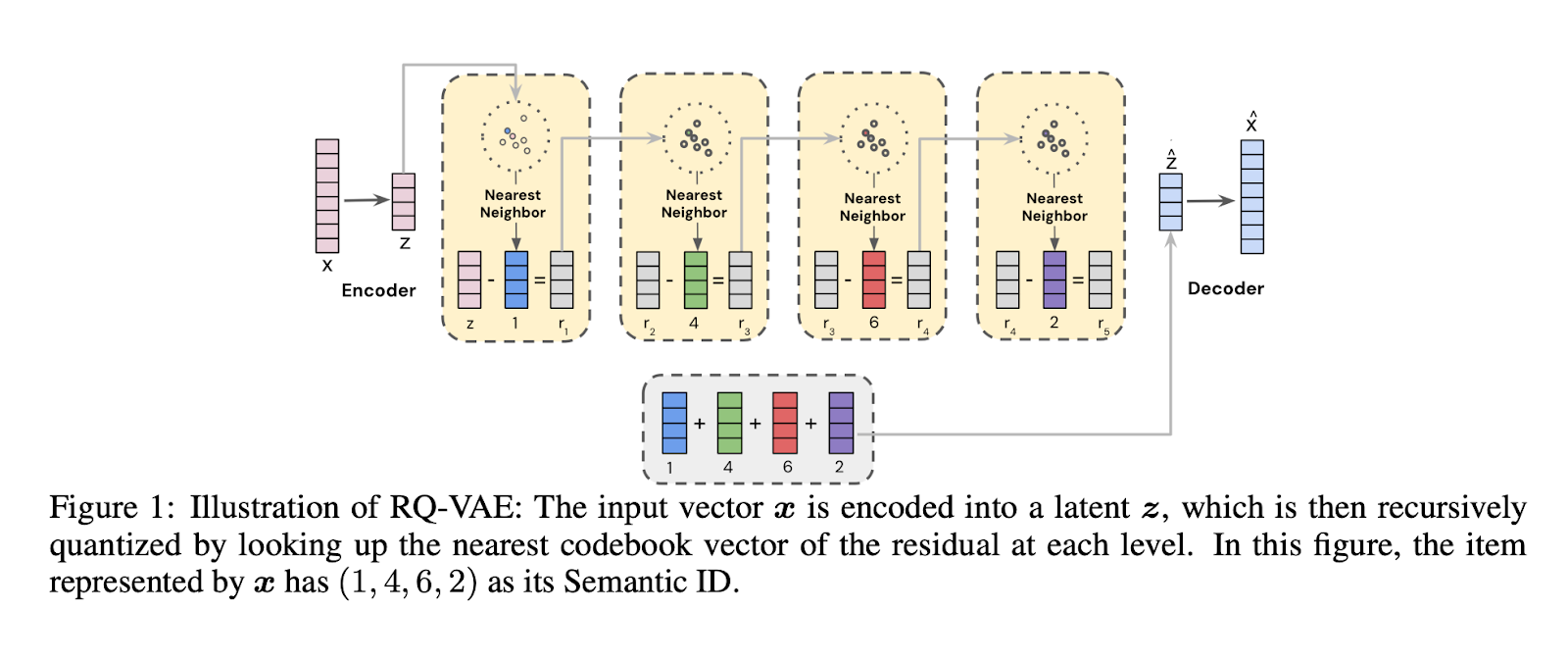
Generative Retrieval & Semantic IDs
To bridge the gap for Transformers, we are currently working on a production implementation of Semantic IDs. Instead of random hashes, we use item metadata to generate a hierarchical “path” via Residual Quantization (RQ-VAE).
This transforms a 100-million-way classification problem into a series of much smaller, manageable 1,024-way classifications (e.g., Category 12 -> Sub-cluster 405 -> Item 8). The goal is to move from Discriminative Ranking to Generative Retrieval, allowing us to maintain the uniqueness required by Transformers while finally deleting the last of our stateful ID maps.
Lessons Learned: Training Lock-in
No engineering solution is a free lunch. While stateless factorization solved our coordination and memory problems, it introduced a new challenge: Training Lock-in.
When you use a standard ID Registry, your system is technically “mutable.” If you want to increase your embedding table from 10 million to 20 million rows, you can write a migration script to re-index your database. It’s painful, but it’s possible.
With stateless factorization, your model is mathematically bound to the specific configuration you chose at the start. The “address” of an ID is a deterministic function of:
- The specific hash algorithm (e.g., MurmurHash3).
- The seed/salt used for that hash.
- The number of tables ($k$).
- The size of each table ($B$).
If you decide six months into production that your collision rate is too high and you want to double your table size from 16,384 to 32,768, you cannot simply “resize” the table. Changing even a single parameter in the hash function completely scrambles the address space. Every ID will now point to a new, random set of weights.
The result: You are forced into a “stop-the-world” retrain. You have to throw away your current weights and train a new model from scratch using the new hashing schema.
This makes the initial choice of “Address Space” a high-stakes architectural decision. At Shaped, we learned to “over-provision” our stateless tables from day one. Using four tables of 16k rows costs us a negligible amount of VRAM (~256 KB), but it provides enough address space (72 Trillion combinations) to ensure we won’t have to scramble our model’s brain as our customers’ catalogs grow from millions to billions of items.
When you move to stateless factorization, you are trading Operational Flexibility for System Scalability. Make sure you choose an address space you can live with for the long haul.
Conclusion: The Death of the Lookup Table
The history of machine learning is the history of moving from Lookup to Compute.
We saw it in NLP when we moved from word-dictionaries to sub-words. We are now seeing it in RecSys. The “Tokenizer Map”, the giant, stateful, fragile database of mappings, is an architectural pattern that doesn’t hold up to the speed of modern infrastructure.
At Shaped, we’ve found that compute is now cheaper than latency. In the time it takes to fetch a single ID from a distributed database like Redis, a GPU can compute a thousand stateless embeddings. If you’re still building a better tokenizer map, you might be fighting the wrong war. It’s time to stop looking up your IDs and start calculating them.
References:
- QR Trick: Meta AI: Compositional Embeddings Using Complementary Partitions (2019)
- DHE: Google Research: Learning to Embed Categorical Features without Embedding Tables (2020)
- Monolith: ByteDance/TikTok: Real-Time Recommendation System With Collisionless Embedding Tables (2022)
- Semantic IDs:Generative Retrieval for Recommendation (2023).
See Shaped in action
Talk to an engineer about your specific use case — search, recommendations, or feed ranking.