If you’ve set up a vector database recently, you’ve seen it. Somewhere in the configuration — maybe when creating an index in Pinecone, or scanning Weaviate’s schema options, or reading Qdrant’s collection settings — there were the four letters HNSW. You probably selected it because it was the default or the recommended option, made a mental note to understand it properly later, and moved on.
This is that article.
Hierarchical Navigable Small World (HNSW) is the approximate nearest neighbor algorithm that powers the fast similarity search layer in most production vector databases today. It’s the reason your semantic search or recommendation system can retrieve the 10 most similar items from a catalog of 10 million in under 10 milliseconds. It’s used at scale by Google, Meta, and Spotify — and it’s the index structure that Shaped builds and manages automatically when you configure vector search in your retrieval engine.
Understanding HNSW is not just academic. The three parameters it exposes — M, ef_construction, and ef — directly control the recall, latency, and memory characteristics of your retrieval system. Getting them wrong means either slow queries or poor results. Getting them right means a retrieval layer that stays out of your way and does its job.
This post explains exactly how HNSW works, what each parameter controls, where the algorithm breaks down, and how it fits into a production retrieval stack.
The problem: finding nearest neighbors at scale
Every vector database is solving the same fundamental problem. You have a collection of items — documents, products, videos, user profiles — each represented as a high-dimensional vector, typically 256 to 1536 dimensions. When a query arrives, you need to find the items whose vectors are most similar to the query vector. That’s nearest neighbor search.
The naive solution is exact: compute the distance from the query to every item in the database and return the closest K. This is called a flat or brute-force index. It’s perfectly accurate. It’s also completely unusable at scale.
Searching one million 768-dimensional vectors with a flat scan takes roughly 2–3 seconds on modern hardware. At 10 million items it takes 20–30 seconds. At the latencies required by real recommendation or search systems — results in under 50 milliseconds — exact search is not viable past a few hundred thousand items.
Approximate nearest neighbor (ANN) search accepts a small, controlled accuracy trade-off in exchange for orders-of-magnitude speed improvements. Instead of finding the provably closest vectors, ANN finds vectors that are very likely to be among the closest — typically achieving 95–99% recall while running 50–200x faster than brute force.
HNSW is the ANN algorithm that, across nearly all realistic workloads in the 1M–100M vector range, achieves the best combination of query speed, recall accuracy, index build time, and memory efficiency.
A brief history of the problem
Understanding why HNSW works requires understanding what came before it.
KD-Trees partition the vector space into a binary tree. They work well in low dimensions (under ~20) but performance degrades exponentially as dimensions increase — the curse of dimensionality. Completely unsuitable for modern embedding models.
Locality-Sensitive Hashing (LSH) hashes similar vectors into the same buckets probabilistically. Fast to build, but achieving high recall requires large hash tables and multiple hash functions. Performance is inconsistent and hard to tune.
Flat / brute-force indexes give perfect recall. Practical only for small corpora or when GPU hardware is dedicated to the task.
Navigable Small World (NSW) graphs, the direct predecessor of HNSW, connect each vector to its approximate nearest neighbors in a graph. To search, you enter the graph at a random point and greedily navigate toward the query — always moving to the neighbor closest to the query vector. NSW works but degrades at scale: navigating from a distant random entry point through a flat graph means traversing many connections before reaching the right neighborhood.
HNSW (Malkov and Yashunin, 2016, published 2018) solves the NSW scaling problem with a single insight: add hierarchy. Build multiple layers of NSW graphs at different densities. Use sparse upper layers for fast coarse navigation, and the dense bottom layer for precise local search. The result is an algorithm with near-constant query time as the index grows.
How HNSW works: the mechanism
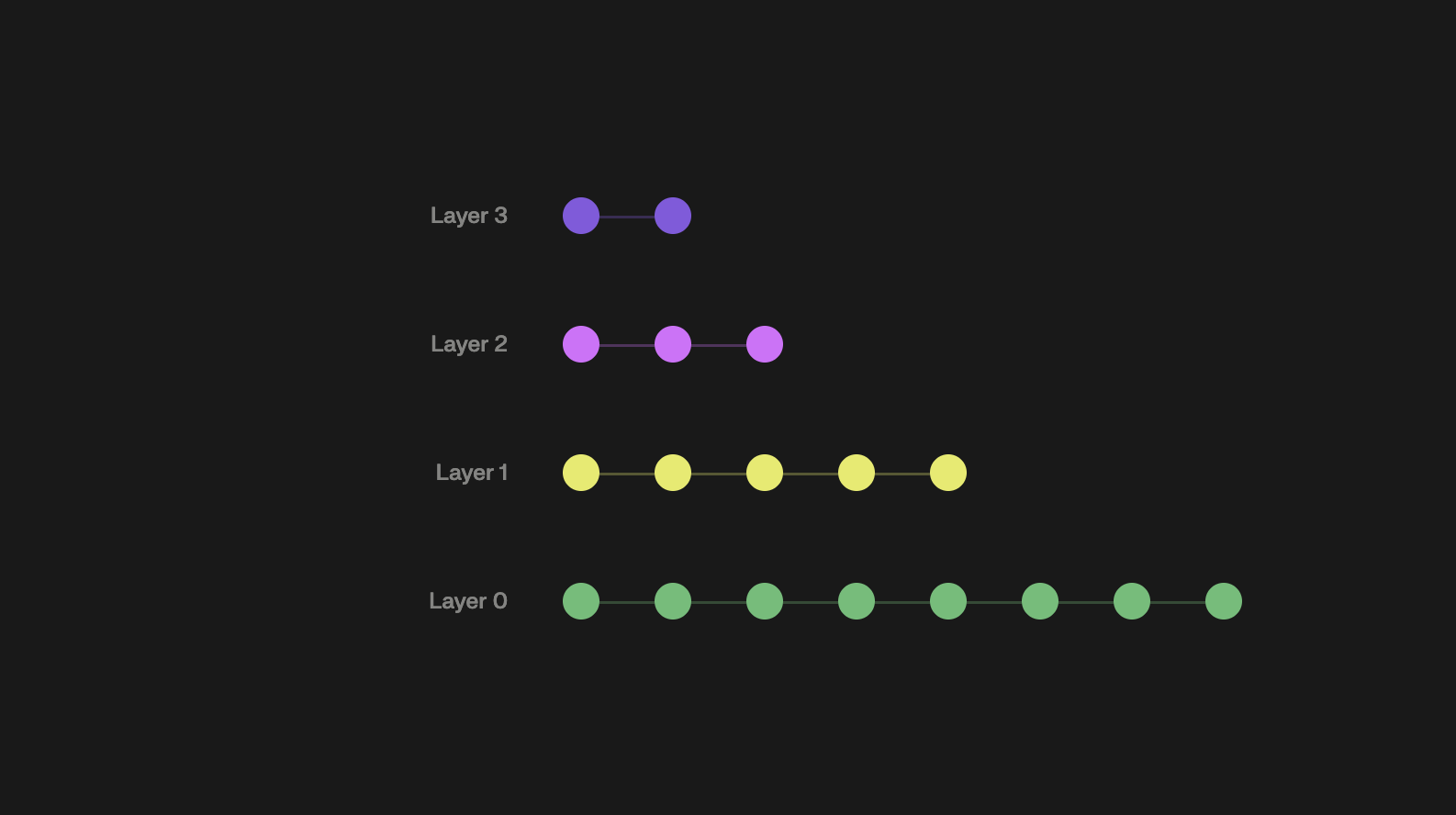
HNSW organises vectors in a multi-layer graph. Each layer is a navigable small world graph. The bottom layer (layer 0) contains every vector with many short-range connections per node. Higher layers contain progressively fewer vectors with longer-range connections — a zoom-out view of the same space.
When a new vector is inserted, it’s randomly assigned a maximum layer (with exponentially decreasing probability for higher layers, so most vectors only exist in layer 0). The algorithm finds the vector’s nearest neighbors at each layer and creates bidirectional links.
Search works in two phases:
Phase 1 — coarse navigation. Enter at the designated entry point at the top layer. Greedily navigate downward: at each layer, move to the neighbor closest to the query, then descend. This runs in O(log n) time — each layer has logarithmically fewer nodes than the one below. Think of it as taking the highway: fast long-distance travel before switching to local streets.
Phase 2 — fine search. Arrive at layer 0 in approximately the right region. Switch to a beam search using a dynamic candidate list of size ef. Explore the local neighborhood thoroughly, maintaining a priority queue of the best candidates seen. Return the top-K.
The hierarchy solves NSW’s scaling problem. Upper layers guide you to the correct region in logarithmic time. The expensive local search only begins once you’re already close to the answer.
A concrete example with actual distances
Abstract explanations of greedy graph navigation are hard to internalise. Here’s a concrete walkthrough.
Imagine querying a 3-layer HNSW index. The query vector Q is at some position in the space. Here’s what the search looks like, with actual distances at each step:
We evaluated roughly 100 nodes total to find the answer in a corpus of 1 million. Brute force would have evaluated all 1 million. That’s the HNSW trade-off in concrete form: a few missed results (items 0.10–0.13 from Q that we didn’t explore) in exchange for a 10,000x reduction in computation.
The three parameters that matter
HNSW exposes three parameters. Every other parameter in a vector database UI is either derived from these or has negligible impact on performance.
M — connections per node
M is the number of bidirectional links each node maintains at layer 0. At higher layers, nodes maintain M/2 links.
Higher M means a denser, more connected graph. More connections mean more paths to the query’s nearest neighbors, which makes it harder for the search to get trapped in a local minimum. This improves recall. It also increases memory usage linearly and index build time.
| M | Use case | Memory overhead vs flat index |
|---|---|---|
| 8–12 | Memory-constrained, lower recall acceptable | ~1.5–2x |
| 16 | Standard default — right for most systems | ~2.5x |
| 32 | High-recall requirements, memory available | ~4x |
| 64+ | Near-exact recall required | ~7x |
The most common mistake: setting M too high. The recall improvement from M=32 to M=64 is marginal while memory doubles. Start at M=16. Only increase if measured recall falls short of your requirements.
ef_construction — build-time search width
ef_construction controls how many candidates are evaluated when finding neighbors during index construction. It determines graph quality.
Higher values produce a better-connected graph and better recall at query time. The cost is longer build time only — once the index is built, ef_construction has zero effect on query latency or memory.
Rule of thumb: ef_construction should be at least 2 * M. Values between 100 and 200 are standard for production. Returns diminish sharply above 400.
This is the parameter teams most often underinvest in, because its effects only appear in production recall metrics rather than anything immediately visible during development. A poorly constructed graph can give you mediocre recall no matter how high you set ef at query time.
ef (ef_search) — query-time search width
ef controls the size of the dynamic candidate list during layer-0 beam search. It must be ≥ k (the number of results requested).
This is the parameter teams get wrong most often — not because they misunderstand it, but because they set it once during development and never revisit it. ef is the primary lever for the recall-speed trade-off in production. Critically, it can be adjusted at query time without rebuilding the index.
ef=10:   fastest queries  ~85-90% recall@10  (acceptable for feeds, not for search)
ef=50:   balanced         ~95-97% recall@10  ← right for most production systems
ef=100:  thorough         ~98%   recall@10
ef=200:  near-exact       ~99.5% recall@10   (slower — justify with use case)
ef=500+: diminishing returns, use brute force instead
For a recommendation feed, 96% recall@10 at ef=50 means 9.6 of the 10 returned items are genuinely in the true top-10. The 0.4 missed are so close in similarity score that the downstream ranking impact is typically invisible to users. For a RAG pipeline where a single missed document causes a hallucination, ef=200 may be justified.
Diagnosing production problems
The question practitioners actually ask isn’t “what does ef do” — it’s “my system has problem X, which parameter do I change?”
| Symptom | Most likely cause | Fix |
|---|---|---|
| Recall too low | ef too small | Increase ef first — no rebuild needed |
| Recall still low after increasing ef | M too small, or poor ef_construction | Rebuild with higher M and ef_construction |
| Queries too slow | ef too large | Decrease ef |
| Index uses too much memory | M too large | Rebuild with lower M |
| Index build too slow | ef_construction too large | Reduce ef_construction (minor recall cost) |
| Recall degrades gradually over time | Index bloat from deletions | Periodic full index rebuilds |
The recall-latency trade-off in practice
Approximate performance for a 1M vector index, 768-dimensional vectors, M=16, ef_construction=200, on modern cloud hardware:
| ef | Recall@10 | Queries/sec | P99 latency |
|---|---|---|---|
| 10 | ~88% | ~8,000 | ~2ms |
| 50 | ~96% | ~3,500 | ~5ms |
| 100 | ~98% | ~2,000 | ~9ms |
| 200 | ~99.5% | ~1,000 | ~18ms |
| Brute force | 100% | ~80 | ~200ms |
HNSW at ef=50 delivers 96% recall at 44x the throughput of brute-force search. The shape of this curve — large gains in throughput for small losses in recall — is what makes HNSW so useful.
How HNSW compares to alternatives
| Algorithm | Query speed | Recall | Memory | Incremental updates | Best for |
|---|---|---|---|---|---|
| HNSW | Very fast | Very high | High | Yes | 1M–100M vectors |
| IVF-Flat (FAISS) | Fast | High | Medium | Batch rebuild only | Large batches, moderate recall |
| IVF-PQ (FAISS) | Very fast | Medium | Low | Batch rebuild only | Billion scale, memory-constrained |
| ScaNN (Google) | Very fast | Very high | Medium | Batch rebuild only | Billion scale, accuracy critical |
| Annoy (Spotify) | Medium | Medium | Medium | No | Static indexes |
| Brute force | Very slow | 100% | Low | Instant | <100K vectors |
HNSW’s key advantage over IVF-based methods is incremental updates. You can add and remove individual vectors without rebuilding the entire index. For recommendation systems where catalogs change constantly, this matters enormously — IVF methods require full rebuilds when the distribution shifts significantly.
HNSW’s main weakness is memory. At billion scale the graph structure requires terabytes of RAM, making distributed deployments or quantization-aware methods (IVF-PQ, ScaNN) necessary. For the 1M–100M range covering most production recommendation and search systems, HNSW is the right default.
Where HNSW breaks down
Memory at billion scale. A 1B vector index with M=16 and 768-dimensional embeddings requires roughly 4–8 TB of RAM. Only viable with distributed HNSW. At billion scale, IVF-PQ or ScaNN with quantization are better choices.
Heavy deletion workloads. HNSW marks deleted nodes as tombstones rather than physically removing them, causing index bloat over time and gradual recall degradation. If 20%+ of your catalog turns over monthly, plan for periodic full index rebuilds.
Skewed distributions. HNSW’s greedy navigation assumes vectors are roughly uniformly distributed. When data clusters heavily — say, 80% of items in a few dense categories — search can get trapped in popular clusters and miss relevant items in sparser regions. Monitor recall segmented by query type, not just average recall across all queries.
HNSW in a production retrieval stack
HNSW handles candidate generation — narrowing a catalog of millions to a manageable set of hundreds for downstream ranking models.
returns ~500 candidates
scores ~200 filtered candidates, ~20ms
HNSW’s job is to make the scoring stage tractable. A LightGBM model scoring 200 candidates is fast. Scoring 10 million is not.
One thing worth stating plainly: HNSW can only find what the embedding model puts near the query vector. If your embeddings represent “comfortable shoes for standing all day” far from items described as “memory foam insoles, orthopedic support” — HNSW will not fix that. The embedding space is upstream of everything. HNSW maximises recall within the space you give it. Getting the embedding space right is at least as important as getting the HNSW parameters right.
From theory to production: Building and maintaining HNSW in production means managing index construction, parameter tuning, incremental updates, distributed serving, and recall monitoring. For a step-by-step guide on deploying production retrieval without that infrastructure burden, read how to deploy a production retrieval system with Shaped in under a week.
HNSW in Shaped: what you configure and what you don’t
When you define an engine with an index.embeddings block in Shaped, the platform builds and manages HNSW indexes over those embeddings automatically — construction, parameter tuning, real-time updates when items change, and serving at sub-50ms latency.
A minimal vector index configuration:
# product_search_engine.yaml
version: v2
name: product_search_engine

data:
  item_table:
    name: products
    type: table

index:
  embeddings:
    - name: product_embedding
      encoder:
        type: hugging_face
        model_name: sentence-transformers/all-MiniLM-L6-v2
        batch_size: 256
        item_fields:
          - title
          - description
          - category
This creates an HNSW index over embeddings generated from your product titles, descriptions, and categories. Shaped handles construction, parameter management, and real-time updates when products change.
You can define multiple embeddings — and therefore multiple HNSW indexes — within a single engine:
# multi_embedding_engine.yaml
index:
  embeddings:
    - name: text_embedding
      encoder:
        type: hugging_face
        model_name: sentence-transformers/all-MiniLM-L6-v2
        batch_size: 256
        item_fields:
          - title
          - description

    - name: visual_embedding
      encoder:
        type: hugging_face
        model_name: openai/clip-vit-base-patch32
        batch_size: 32
        item_fields:
          - image_url

    - name: collab_embedding
      encoder:
        type: trained_model
        model_ref: als_score       # trained on your interaction data
Three HNSW indexes — text, visual, collaborative — queryable independently or combined at runtime via ShapedQL:
-- multi_embedding_query.sql
SELECT item_id, title, price
FROM
  text_search($query,
    mode='vector',
    text_embedding_ref='text_embedding',
    limit=200),                              -- HNSW over text embeddings
  similarity(
    embedding_ref='collab_embedding',
    input_user_id=$user_id,
    limit=200)                               -- HNSW over collaborative embeddings
WHERE in_stock = true
  AND price <= $max_price
ORDER BY relevance(user, item)
LIMIT 10
Each text_search(mode='vector') and similarity() call is an HNSW query. Results from both indexes are merged, filtered by business rules, and scored by the ranking model. The final result benefits from both semantic relevance to the query and personalisation to the specific user — something neither index alone provides.
What Shaped abstracts away: index construction, HNSW parameter selection, incremental updates when items change, distributed serving infrastructure, and recall monitoring over time.
Measuring HNSW index quality in production
Two metrics matter:
Recall@k — of the true top-k nearest neighbors, what fraction does HNSW return? Measure this by running sample queries against both HNSW and brute-force and comparing result sets. A production index should achieve at least 95% recall@10 for most applications. Below 90% usually means ef is too low or M is too small.
P99 query latency — not mean latency. You care about the tail, not the average. If your P99 is within budget, the mean is fine.
Track both over time. Recall can degrade gradually as items are deleted and the index accumulates tombstones, or as the item distribution shifts away from what the graph was optimised for.
Summary
HNSW works because of hierarchy. Sparse upper layers for fast coarse navigation. Dense bottom layer for precise local search. The result: an algorithm that behaves like a highway system for your vector space — express lanes to the right neighborhood, local streets for the final precise search.
The three parameters control distinct trade-offs: M sets graph density before build, ef_construction sets index quality at build time, and ef sets the recall-speed trade-off at query time — the only one you can change without a rebuild.
In production, HNSW is one component of a larger pipeline. It generates candidates fast enough that accurate downstream ranking models have time to do their job. The ceiling on retrieval quality is set by your embedding space, not by HNSW. Getting the embeddings right is upstream of everything else.
If you want HNSW-powered vector retrieval in production without managing the index infrastructure, Shaped handles the full lifecycle automatically — you declare what to embed, and the platform takes care of the rest.
Further reading
- Malkov and Yashunin, “Efficient and robust approximate nearest neighbor search using Hierarchical Navigable Small World graphs” (2018) — the original HNSW paper
- The Two-Tower Model for Recommendation Systems: A Deep Dive — how two-tower models generate the embeddings that HNSW indexes
- Cosine Similarity is Not the Silver Bullet — why the distance metric you use with HNSW matters
- Vector Search: Lucene is All You Need — practical vector search trade-offs in production
- The Anatomy of Modern Ranking Architectures — where HNSW fits in a complete retrieval pipeline
See Shaped in action
Talk to an engineer about your specific use case — search, recommendations, or feed ranking.