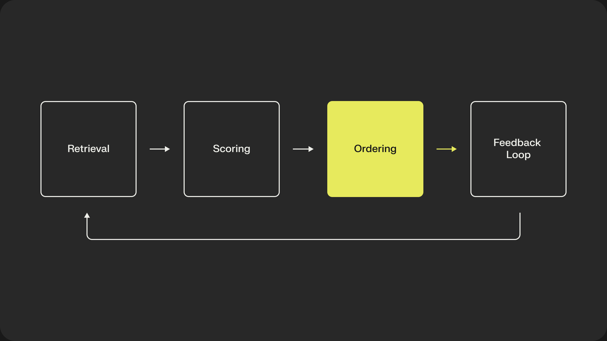
The Ordering Stage: From Scores to a Final Page

1. In Part 1, we established the multi-stage architecture.
2. In Part 2, we covered the Retrieval Stage, where we generated a high-recall candidate set.
3. In Part 3, we dove into the Scoring Stage, where we assigned precise, pointwise scores to each of those candidates.

At the end of the last stage, we were left with a list of roughly a thousand candidate items, each with one or more independent scores (e.g., p(click), expected_watch_time). A naive approach would be to simply sort this list by our primary score and call it a day.

This is a common mistake that separates a basic recommender from a production-grade system. A simple sorted list is not a product. It often leads to a monotonous, unengaging, and commercially suboptimal user experience.

The Ordering Stage is the final, crucial mile. Its job is to take the raw, scored candidates and apply listwise logic to construct the final page or feed. This is where machine learning predictions meet product design, business rules, and a holistic view of the user experience. The thinking shifts from "how good is this one item?" (pointwise) to "how good is this set of items together?" (listwise).

The Problem with a Simple Sort: Homogeneity and Filter Bubbles

If you sort a list of YouTube video recommendations purely by predicted click-through rate, you will likely get ten videos from the same creator on the same topic. If you sort an e-commerce catalog purely by p(purchase), you might see ten nearly identical-looking black t-shirts.

This is because the scoring model, working pointwise, correctly identifies that if a user is likely to engage with one of these items, they are probably likely to engage with all of them. But showing a user ten of the same thing is a terrible experience. This is the homogeneity problem, and it's the first thing the Ordering Stage must solve.

Enforcing Diversity with Maximal Marginal Relevance (MMR)

The most common and effective algorithm for solving this is Maximal Marginal Relevance (MMR). The intuition is simple: we want to build our final ranked list greedily, one item at a time. At each step, we select the item that offers the best trade-off between its individual relevance and its novelty compared to the items we've already selected.

MMR is defined by the following formula for selecting the next item i from the set of unselected candidates C:

MMR(i) = λ * Score(i) - (1 - λ) * max_{j ∈ S} Similarity(i, j)

Let's break this down:

• Score(i): The original relevance score from our scoring model.
• Similarity(i, j): A measure of similarity between candidate item i and an already selected item j. This is often the cosine similarity of their item embeddings.
• S: The set of items already selected for our final list.
• λ (lambda): A tuning parameter between 0 and 1 that controls the trade-off.
  
  • If λ = 1, the formula ignores similarity, and we're back to a simple sort by score.
  • If λ = 0, the formula ignores relevance and picks the most dissimilar items, which is not what we want.
  • A typical value is around λ = 0.7, which prioritizes relevance but applies a penalty for redundancy.

Here is a simple, clear Python implementation of the MMR algorithm:

1 import numpy as np
2 from sklearn.metrics.pairwise import cosine_similarity
3 
4 def maximal_marginal_relevance(
5     candidate_embeddings: np.ndarray,
6     candidate_scores: np.ndarray,
7     selected_indices: list,
8     lambda_param: float = 0.7,
9     top_k: int = 10
10 ) -> list:
11     """
12     Performs Maximal Marginal Relevance to re-rank a list of candidates.
13     Args:
14         candidate_embeddings (np.ndarray): Embeddings for all candidate items.
15         candidate_scores (np.ndarray): Original relevance scores for all candidates.
16         selected_indices (list): The list of indices already selected (can start empty).
17         lambda_param (float): The trade-off parameter between relevance and diversity.
18         top_k (int): The number of items to select for the final list.
19     Returns:
20         list: A list of indices representing the re-ranked items.
21     """
22     num_candidates = len(candidate_scores)
23     remaining_indices = list(set(range(num_candidates)) - set(selected_indices))
24 
25     while len(selected_indices) < top_k and remaining_indices:
26         mmr_scores = {}
27 
28         for i in remaining_indices:
29             relevance_score = candidate_scores[i]
30 
31             if not selected_indices:
32                 diversity_penalty = 0
33             else:
34                 selected_embeddings = candidate_embeddings[selected_indices]
35                 candidate_embedding = candidate_embeddings[i].reshape(1, -1)
36                 similarity_with_selected = cosine_similarity(candidate_embedding, selected_embeddings)
37                 diversity_penalty = np.max(similarity_with_selected)
38 
39             mmr_scores[i] = lambda_param * relevance_score - (1 - lambda_param) * diversity_penalty
40 
41         best_candidate_index = max(mmr_scores, key=mmr_scores.get)
42         selected_indices.append(best_candidate_index)
43         remaining_indices.remove(best_candidate_index)
44 
45     return selected_indices

The Explore-Exploit Trade-off: Surfacing New and Uncertain Items

The models and algorithms we've discussed so far are masters of exploitation. They are designed to exploit known user preferences and item characteristics to predict the most likely positive outcomes. If a user has clicked on 10 sci-fi movie recommendations, the model will confidently predict they will click on an 11th.

If left unchecked, this pure exploitation leads to two severe problems:

1. User Monotony: The user gets stuck in a "filter bubble," only ever seeing recommendations similar to what they've engaged with in the past. We never discover if their interests have evolved or if they might enjoy a different genre.
2. Item Starvation & Feedback Loops: New items, which have no interaction data, will receive very low scores from the scoring model. They will never be surfaced, never gather interactions, and therefore will always have low scores. The system creates a self-fulfilling prophecy where only popular items stay popular. This is a classic feedback loop.

The Ordering Stage is where we must explicitly break this loop by injecting exploration. We need to intelligently surface items that the model is uncertain about, giving them a chance to be seen and gather data.

Here are a few common, practical strategies for managing the explore-exploit trade-off.

Strategy 1: Score Boosting and Heuristics

The simplest method is to apply a heuristic "boost" to the scores of new or under-exposed items.

• Age-Based Boosting:
• A common formula is to add a bonus to an item's score that decays with its age or the number of impressions it has received. final_score = model_score + w_boost * exp(-decay_rate * item_age_in_hours)

This gives new items a temporary lift, allowing them to compete with established items. The w_boost and decay_rate are hyperparameters that are tuned to control how aggressively the system explores.

• Cold-Start Slots: A variation on this is to use the "slotting" technique we'll discuss later to reserve specific slots in the ranking for new items (e.g., "always show one item from the 'New Arrivals' retriever in the top 10").

Strategy 2: Probabilistic Exploration - Thompson Sampling

A more principled approach is to use a probabilistic method that naturally balances exploration and exploitation. Thompson Sampling is a powerful and elegant algorithm for this.

The intuition is to treat the predicted score not as a single point estimate, but as a probability distribution. For example, instead of our model predicting that p(click) = 0.05, we can model this prediction as a Beta distribution, which is defined by two parameters: alpha (successes, e.g., clicks) and beta (failures, e.g., non-clicks).

The ranking process at request time then becomes:

1. For each candidate item, we have its historical alpha (total clicks) and beta (total impressions - clicks).
2. Instead of using the average score (`alpha / (alpha + beta)`), we draw a random sample from each item's Beta distribution: sampled_score = Beta.sample(alpha + 1, beta + 1).
3. We then rank all candidates based on these sampled_score values.

This has a beautiful emergent property:

• For well-known items (high alpha, high beta): The Beta distribution is very narrow and peaked around its true mean. The sampled score will be very close to the historical CTR, so we exploit.
• For new or uncertain items (low alpha, low beta): The Beta distribution is very wide and flat. The sampled score could be anywhere from very low to very high. This gives uncertain items a "chance to be lucky" and get ranked highly, allowing them to explore.

As an uncertain item gets more impressions, its distribution narrows, and the system will naturally either exploit it (if it's good) or ignore it (if it's bad).

Strategy 3: Uncertainty-Based Exploration - Upper Confidence Bound (UCB)

Another popular method is Upper Confidence Bound (UCB). Instead of sampling, UCB calculates an optimistic "potential score" for each item and ranks by that.

The formula is typically of the form:

UCB_score = mean_score + exploration_bonus exploration_bonus = C * sqrt(log(total_impressions) / (item_impressions + epsilon))

Let's break this down:

• mean_score: The historical, observed score for the item (the "exploit" term).
• exploration_bonus: This is the "explore" term. It is highest for items that have been seen very few times (item_impressions is low) relative to the total number of requests. The constant C controls how much we value exploration.

UCB effectively says, "Let's rank by the upper end of the confidence interval for each item's true score." Like Thompson Sampling, this gives a natural boost to new and uncertain items.

Injecting one of these exploration strategies into the ordering stage is non-negotiable for building a healthy, adaptive recommender system. It's the primary mechanism we have to gather new training data, discover new user interests, and prevent our models from getting stuck in the past.

Blending and Interleaving: Weaving the DAG Back Together

As we discussed in Part 1, a production system generates candidates from multiple sources (the "ensemble of retrievers"). The Scoring Stage then produces scored lists for each source. This leaves us with a new problem: the scores are not comparable. A p(click)=0.8 from a mature organic model is not the same as a score from a cold-start model or a bid_price from an ad server.

The Ordering Stage is responsible for merging these disparate lists into a single, coherent ranking. Common strategies include:

1. Heuristic Normalization: A simple but brittle approach is to try and normalize all scores to a common scale (e.g., 0-1) and then sort. This often fails because the score distributions from different models can vary wildly.
2. Dedicated Blending Model: A more sophisticated approach is to train a second-level model that takes the scores from all the first-level models as features and learns the optimal way to combine them. This is powerful but adds complexity.
3. Slotting and Templating: This is the most common and robust pattern in production. The final page is treated as a template with pre-defined slots. Business logic determines how to fill these slots. For example:
   
   • Slot 1: Pinned promotional banner.
   • Slots 2, 3, 5: Top organic results.
   • Slot 4: Top ad result.
   • Slot 6: Top result from a "New and Trending" retriever to ensure freshness.

The Final Polish: Applying Business Logic and Page Construction

The final step in the Ordering Stage is to apply a layer of hard-coded business rules and assemble the final page. This is where the recommender system truly becomes a product.

These rules are often non-negotiable and override any model's prediction:

• Pinning: Forcing a specific item (like a major movie release or a site-wide announcement) to the top position.
• Content Pacing: Enforcing rules like "don't show more than two videos from the same creator in the first ten results."
• Deduplication: Ensuring an item doesn't appear in multiple carousels on the same page.
• Page Assembly: For complex UIs like the Netflix homepage, the Ordering Stage is responsible for assembling the entire page. It doesn't just produce one list; it produces many lists, one for each carousel ("Trending Now," "Because You Watched...", etc.), and delivers them as a single, structured response.

Tying it All Together: The Online Ordering Flow

Here is a simplified pseudo-code block showing how these components work together in the online path:

import numpy as np

def order_and_construct_page(scored_candidate_sets, user_context):
    """
    Applies listwise logic to build the final page.
    Args:
        scored_candidate_sets (dict): A dict like 
            {'organic': [(item_id, score), ...], 'ads': [(item_id, score), ...]}
    """
    final_ranked_ids = []

    # --- 1. Blending & Interleaving (using a slotting approach) ---
    page_template = ["ORGANIC", "ORGANIC", "AD", "ORGANIC", "NEW_CONTENT"]

    organic_candidates = iter(scored_candidate_sets.get('organic', []))
    ad_candidates = iter(scored_candidate_sets.get('ads', []))
    new_content_candidates = iter(scored_candidate_sets.get('new_content', []))

    unranked_pool = []
    for slot_type in page_template:
        if slot_type == "ORGANIC":
            unranked_pool.append(next(organic_candidates, None))
        elif slot_type == "AD":
            unranked_pool.append(next(ad_candidates, None))
        elif slot_type == "NEW_CONTENT":
            unranked_pool.append(next(new_content_candidates, None))

    # Filter out any None values if iterators were exhausted
    unranked_pool = [item for item in unranked_pool if item is not None]

    # --- 2. Apply Diversity (MMR) ---
    # We need embeddings and scores for the items in our pool
    pool_ids = [item[0] for item in unranked_pool]
    pool_scores = np.array([item[1] for item in unranked_pool])
    pool_embeddings = get_embeddings_for_ids(pool_ids) # Assume a helper function

    diverse_ranked_indices = maximal_marginal_relevance(
        pool_embeddings, pool_scores, [], lambda_param=0.7, top_k=len(pool_ids)
    )
    final_ranked_ids = [pool_ids[i] for i in diverse_ranked_indices]

    # --- 3. Apply Final Business Logic ---
    # Example: Pin a specific promotional item to the top
    promo_item_id = 12345
    if promo_item_id in final_ranked_ids:
        final_ranked_ids.remove(promo_item_id)
    final_ranked_ids.insert(0, promo_item_id)

    # Apply content pacing, deduplication, etc.
    final_ranked_ids = apply_pacing_rules(final_ranked_ids)

    return final_ranked_ids

Conclusion

The Ordering Stage is the crucial final translator between raw model predictions and a polished user experience. It takes a list of independently scored items and applies listwise logic—enforcing diversity, blending multiple sources, and applying business rules—to construct a final ranking that is coherent, engaging, and aligned with product goals.

We have now followed a single request from the initial billions of items all the way to a final, ordered list. But how does the system learn and improve? How do we know if our changes are actually making the product better?

In our final post, we'll close the loop and explore the Feedback and Evaluation Engine that powers the entire system's learning cycle.