
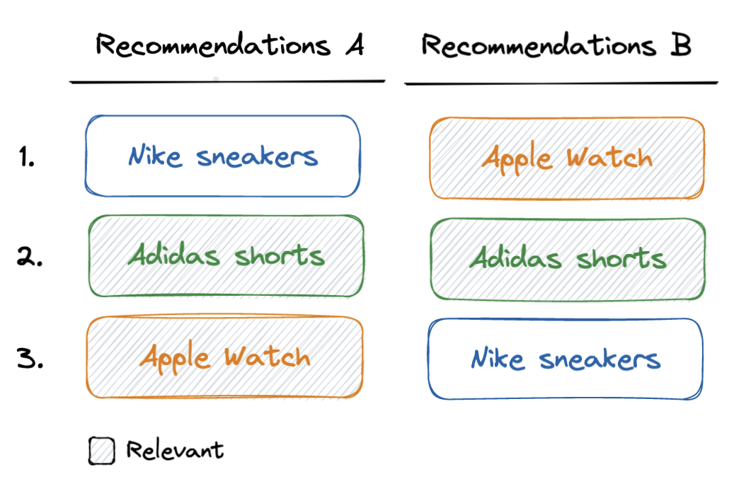
Considering both of these lists have the same items, the question of relevance becomes a question of what order is best. Typically we assume the more relevant list is the one that has more relevant items closer to the top/start of the list. This is because for feed like use-cases where an item is surfaced one after an other (e.g. like TikTok), it’s important that the top items of the feed are the most relevant to keep the user engaged. It’s equally important for carousel recommendation use-cases (e.g. like Netflix), where the items to the left of the carousel are often the first looked at as the audience gazes of the page.
In our first post on evaluating recommendation systems we looked at evaluating Precision@k, Recall@k and R-Precision metrics using a test set of relevant items. If you compute them for the example two recommendation feeds, you’ll see they’re not too useful — they’re equivalent for both lists. This is because they’re not capturing anything about the relative order of the rankings, only how many relevant matches are found. Below we discuss two evaluation metrics that are typically used for recommendation system use-cases where ranking order is important.
To motivate these metrics, let’s assume a user has actually purchased: Apple watch, and Adidas shorts, and we’ve put these items in a test set that wasn’t used when training the recommendation algorithms.
Mean Average Precision (mAP)
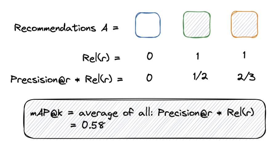
Mean average precision [1] averages the precision@k metric at each relevant item position in the recommendation list. For recommendation list A and using our example user, the relevant items are at position 2 and 3. Therefore, we compute precision@2 and precision@3 and average the results. The mAP values for algorithm A and B are below:
- Algorithm A, mAP = (precision@2 + precision@3) / 2 = (1/2 + 2/3) / 2 = 0.58
- Algorithm B, mAP = (precision@1 + precision@2) / 2 = ( 1/1 + 2/2) / 2 = 1
As you can see from the example, this metric rewards the recommendation algorithm that puts more items at the top of the list. This is because any non-relevant items at the start of the list are factored into the aggregation at each subsequent precision@r computation.
 Mean Average Precision (mAP).Where Rel(r) is an indicator that specifies whether the item at rank r is relevant. Note that the normalization factor of the varge can either be the total number of recommendations or the total number of relevant items (or the minimum of both).
Mean Reciprocal Rank (MRR)
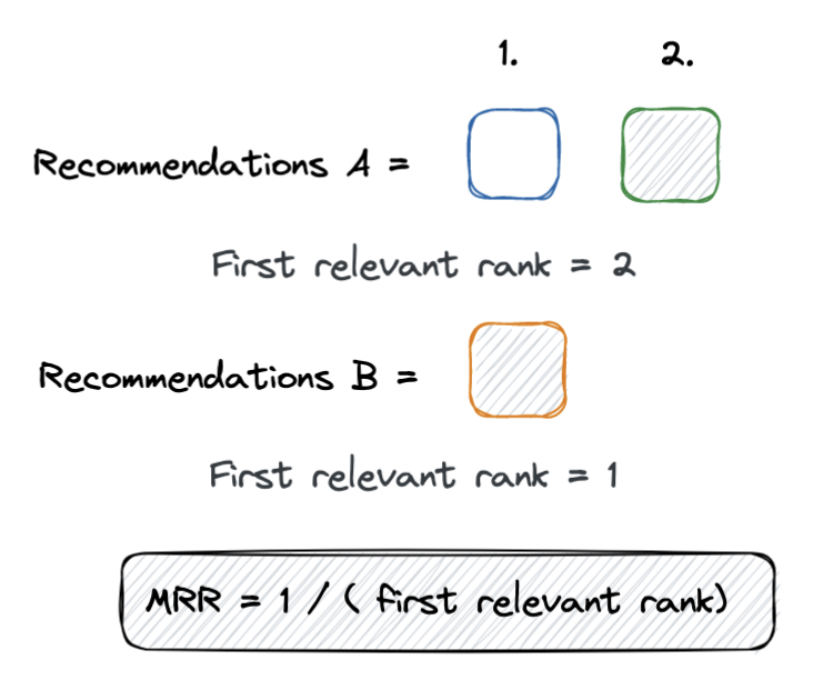
Mean Reciprocal Rank quantifies the rank of the first relevant item found in the recommendation list. The only complexity is that it takes the reciprocal of this “first relevant item rank”, meaning that if the first item is relevant (i.e. the ideal case) then MRR will be 1, otherwise it’ll be lower. For the example above, the first recommendation list has a first relevant item at rank 2 (Adidas shorts). The second recommendation list has a relevant item at rank 1 (Apple watch). Therefore:
- Algorithm A, MRR = 1/2 = 0.5
- Algorithm B, MRR = 1/1 = 1
 Mean Reciprocal Rank (MRR)
Normalized Discounted Cumulative Gain (NDCG)
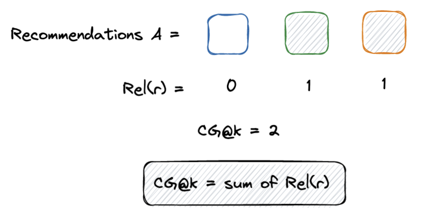
Normalized Discounted Cumulative Gainis the other commonly used ranking metric. Its best explained by first defining Cumulative Gain (CG) as the sum of relevant items among top k results. Note that this value for the binary case is the numerator of Precision@k and Recall@k and doesn’t take into account any ordering.
 Cumulative Gain (CG)
*Discounted Cumulative Gain (DCG)*is where the ordering comes into play. This metric discounts the “value” of each of the relevant items based on its rank. The problem with DCG, is that even an “ideal” recommendation algorithm won’t always be able to get DCG@k = 1.
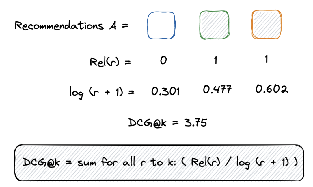 Discounted Cumulative Gain (DCG)
*Normalized DCG (NDCG),*the final iteration, it normalizes DCG by the “ideal” recommendation algorithm (IDCG@k). That is, an algorithm where every relevant item is ranked at the start of the list.
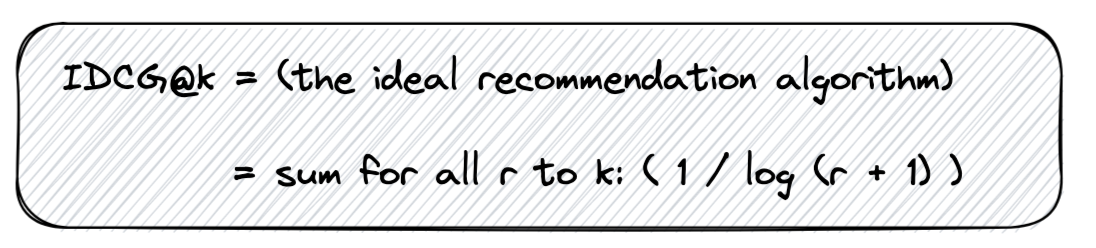 IDCG@k
 NDCG@k
So looking at our example user, lets compute NDCG@k for both recommendation lists. We can first compute IDCG because it’s a constant: IDCG@k = (1/log(1 + 1) + 1/log(2 + 1)) = 5.417. Then we’ll compute DCG and put it altogether for each algorithm:
Algorithm A:
- DCG@k = 1/log(2 + 1) + 1/log(3 + 1) = 3.756
- NDCG@k = NDCG@k / IDCG@k = 0.693
Algorithm B:
- DCG@k = 1/log(1 + 1) + 1/log(2 + 1) = 5.417
- NDCG@k = DCG@k / IDCG@k = 1
As you can see, Algorithm A has a higher NDCG@k, which is what we should expect!
mAP or NDCG?
mAP and NDCG seem like they have everything for this use-case — they both take all relevant items into account, and the order in which they are ranked. However, where MRR beats them across the board is interpretability. MRR gives an indication of the average rank of your algorithm, which can be a helpful way of communicating when a user is most likely to see their first relevant item using your algorithm. Furthermore, MRR might map better to your final use-case better, for example if you care more about the “I’m Feeling Lucky” search result, than the standard “Search” ranking.
When should we use mAP vs NDCG? mAP has some interpretability characteristics in that it represents the area under the Precision-Recall curve. NDCG is hard to interpret because of the seemingly arbitrary log discount within the DCG equation. The advantage of NDCG is that it can be extended to use-cases when numerical relevancy is provided for each item.
NDCG with relevance
To motivate where NDCG reigns supreme, let’s say we have another user who has previously purchased: 1x Apple watch, 5x Adidas shorts and 3x Nike sneakers. We may conclude that the relevancy of each item is weighted by how many items were purchased. So let’s define:
- relevance(Apple watch) = 1
- relevance(Adidas shorts) = 5
- relevance(Nike sneakers) = 3
Then recomputing the NDCG metrics:
IDCG@k = 5/log(1 + 1) + 3/log(2 + 1) + 1/log(3 + 1) = 24.55
Algorithm A:
- DCG@k = 3/log(1 + 1) + 5/log(2 + 1) + 1/log(3 + 1) = 22.104
- NDCG@k = DCG@k / IDCG@k = 0.9
Algorithm B:
- DCG@k = 1/log(1 + 1) + 5/log(2 + 1) + 3/log(3 + 1) = 18.78
- NDCG@k = NDCG@k / IDCG@k = 0.764
Therefore, we can see that Algorithm A is better in this case.
Note that unfortunately obtaining this ‘ground-truth’ relevance score in practice can be tricky so you don’t see it used as much in practice.
Next steps
Finally, mAP, MMR, and NDCG are great offline metrics for evaluating recommendation algorithm relevancy given historical data but what about measuring these algorithms in the online production setting? Furthermore, what about evaluating more than just relevancy? You may want to ensure your algorithms aren’t biased, surface a diverse range of items and optimize for differently for different actors on your platform. We’ll dive into these questions in the next posts. Stay tuned!
Footer
- For simplicity of the post we’re defining the average precision (AP) metric as the mean average precision (mAP). The only difference is that the mean will compute AP over all users in the test set.
See Shaped in action
Talk to an engineer about your specific use case — search, recommendations, or feed ranking.